The latest Illumina sequencers muddle samples
Introduction
Recently the popular technology and science magazine Wired ran a story discussing a problem with a new model of DNA sequencer. The article chronicled the experiences of a Stanford-based researcher who appeared to be making interesting findings while investigating blood stem cells. Initial optimism turned sour however, as it became clear that potentially significant results were the by-product of a problem with the sequencing technology, causing different samples to become mixed-up on the sequencer. While this was unfortunate, to say the least, for the scientist concerned (who reportedly lost a year’s worth of work), the implications of this technical problem set alarm bells ringing in the wider molecular biology and genomics communities.
The fact that a news outlet such as Wired covered this story pays testament to the potential impact of these findings. Although Wired has a technological focus, it is a publication intended to be of interest and intelligible to a general audience, and so it may be surprising to find a story about sequencing artefacts within its pages. The relevance of the story lay in the fact that the machine used was the latest technology offering from Illumina, the San Diego-based company seen as synonymous with sequencing by many in Life Sciences research. Indeed, the wide-scale use of these machines has left countless researchers worried that their work may be rendered invalid, with key findings in published work or current research programs simply being the result of Illumina machines muddling samples.
The Symptoms
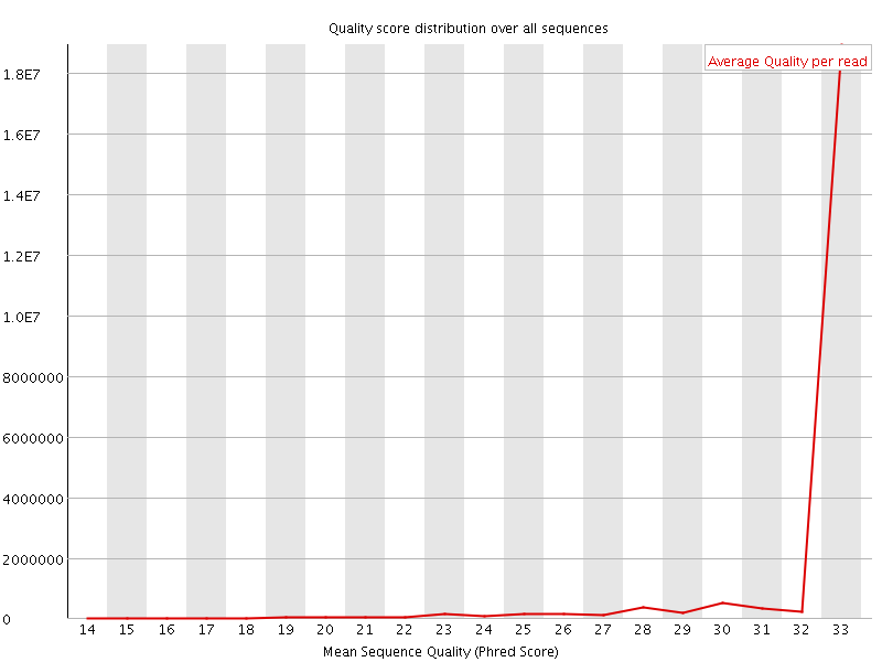
The Stanford researchers deposited their findings on the bioRᵡiv preprint server. Their paper reported that they sequenced mouse single-cell RNA-Seq samples using a HiSeq 4000. As is common when working with single-cell data, they multiplexed the samples: a technique in which DNA molecules are labelled at either end with predefined barcodes, and then the DNA from different libraries are combined. This pool of samples and accompanying barcodes are then sequenced togehter, resulting FASTQ files may be “de-multiplexed” using specialist software, enabling researchers to deduce which read came from what library.
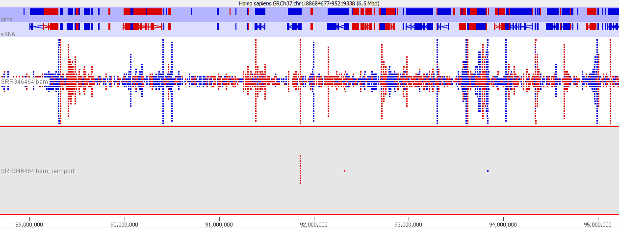
Suspicions were raised when investigating the spatial arrangement of expression patterns between samples on the 384-well plate used during sample preparation. Each well should have contained the cDNA from a single cell, and the samples should have been randomly distributed across the wells. Surprisingly, if a given gene was expressed at very high levels in a particular well, the signal was also detected – but at lower levels – in all or most wells in the same row and column, forming a characteristic cross-like expression pattern in the plot (see figure). Similar patterns could be observed when analysing other types of library e.g. ATAC-Seq. The researchers decided the pattern was most consistent with a being a technical artefact.
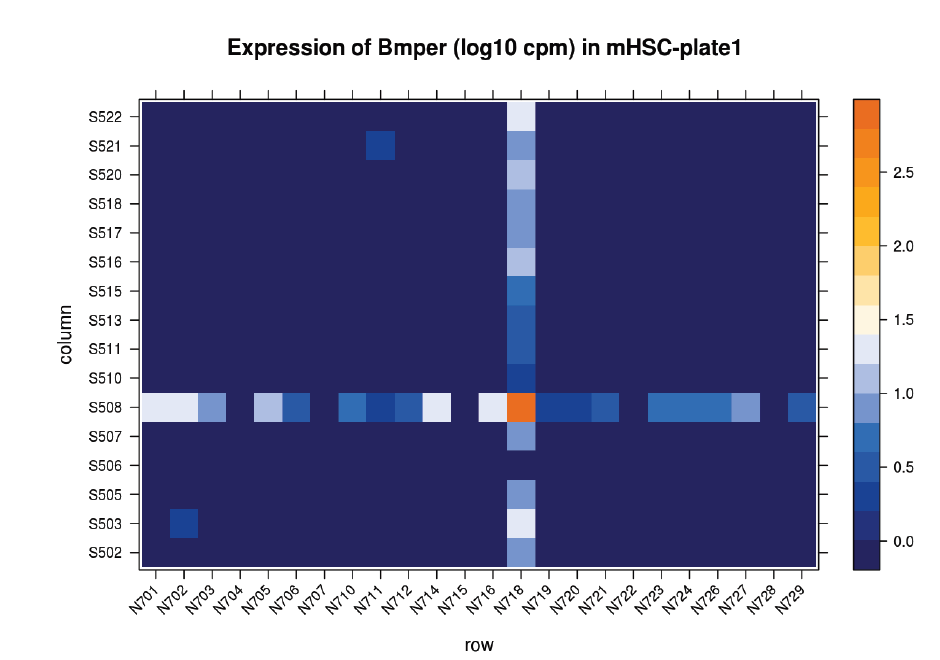
Each row and column correspond to different barcodes. The results show that Bmper is highly expressed in the single-cell sample barcoded with S508/N717. However, almost all the other samples with one of these barcodes also show elevated expression of Bmper. (Taken from bioRᵡiv.)
Diagnosis
The Stanford group re-sequenced their samples on another HiSeq 4000 and observed the same pattern, however the pattern was not observed when sequencing on a NextSeq 500. This was highly significant since the older model NextSeq 500 did not use patterned flowcells, suggesting the problem was specific to that patterned design. This patterned arrangement comprised billions of fixed-sized nanowells distributed uniformly across a sequencing flow cell, enabling the discrimination of separate DNA clusters at much higher densities than possible on previous generation machines.
The cruciform pattern of the mixed signal, which corresponded to the barcode allocation, suggest that one of the barcodes was being mis-identified. To investigate this further they performed an experiment in which wells were allocated either:
- cDNA / reagents (including index primers)
- Reagents (including index primers) only
- No cDNA / no reagents
Barcoded reads corresponding to wells containing neither reagents nor cDNA were very rare. In stark contrast, many reads (around 7% of the average for wells containing cDNA) were found in the wells missing only cDNA. Moreover, these reads mapped to the mouse genome (mm10) with around 80% efficiency. This suggests that the presence of index primers caused the mixing of the sample and consequently when handling multiplexed samples there will be a substantial mix of signals, referred to as “index hopping” or “barcode swapping”.
While the percentages are unsettling, other researchers have reported observing the same phenomenon, but at a significantly reduced level. James Hadfield, the Head of Genomics at CRUK Cambridge Institute, observed an index swapping at rate of around 0.1-0.2% which may not prove so problematic for most applications.
(In fact, a very low level of barcode swapping had been observed on the previous-generation non-patterned machines, but this level should only be a significant problem if mixing greatly differing samples e.g. combining RNA-Seq with ChIP-Seq samples.)
Prevention
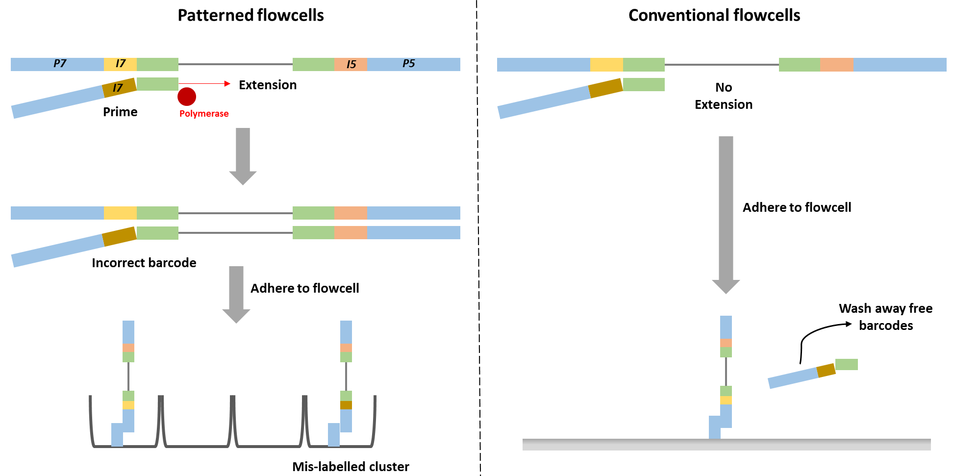
Barcode swapping observed on the HiSeq 4000 was probably a result of the new design using patterned flowcells, and therefore probably should be expected to also occur on the HiSeq 3000 and HiSeq X Ten and the flagship NovaSeq machine. The use of patterned flowcells necessitates the need for a new type of sequencing chemistry, called exclusion amplification (ExAmp), replacing the cluster generation by bridge amplification used on the conventional non-patterned flow cell.
Technical details describing the new sequencing chemistry have not been made publicly available, but examination of the associated patents made it possible to understand the overall process and it is reasonable to assume therefore that index hopping occurs before cluster generation, since all the reagents needed for cluster generation are present in that reaction mix. Free index primers in that mix have the potential to prime library fragments and be extended by DNA polymerase. These molecules, incorrectly assigned barcodes, are free to generate DNA clusters. This is not the case for the conventional flowcell design in which free barcodes are washed away after the DNA is hybridised to the flowcell. Only after this step is DNA polymerase added and sequence extension can initiate.
It is not clear at present how to implement a general purpose bioinformatics solution to remove such artefacts post-sequencing, and indeed experimental solutions may only be possible. To combat the problem, when working with a small number of samples, researchers should stop employing a single-barcode strategy, but instead should double-barcode samples. Following sequencing, reads should then be filtered to allow only those in which both barcodes are identical and have an expected sequence. Since double-barcode swapping should be a rare event, taking this step should greatly reduce sample misclassification.
When multiplexing many samples (already requiring double-barcoding, irrespective of the barcode hopping issue), Stanford researchers advised using barcode pairs in which each individual single barcode was used only once. Although that strategy reduced the number of available barcode combinations, it still allowed many samples to be run on the same lane. In addition, they proposed purification strategies to remove free primers from the library pool.
Illumina recently published a paper confirming the occurrence of index-hopping. They stated that with the proper clean-up of primers and implementing other experimental techniques, it should be possible to minimise barcode swapping to negligible levels for most applications. The report also advised only multiplexing similar conditions in a single lanes. A brain vs liver RNA-Seq example was given in which a transcript is present in liver at a high level, but not at all in the brain. Owing to index hopping that transcript may actually appear to be expressed at a low level in the brain. Illumina suggests that by only combining similar samples (i.e. either brain or liver) in a lane this problem will be prevented. This is far from an ideal solution however, since researchers will need to know in advance what to expect with regard to the expression profiles of their samples and furthermore this strategy would compound the problem of batch effects.
Lessons Learnt
Typically, our QC Fail articles report and analyse data generated in-house, at the Babraham Institute. For this article we have been unable to do this since our institute has not purchased a sequencer with the patterned flow cell design. Rather, we have provided a precis of the investigations of other teams.
Although we have been unable to actively contribute to the community’s knowledge by troubleshooting this problem directly, we, fortunately, have not been placed in the unenviable position of having to decide what sample may or may not have been affected by this problem and re-assessing results in light of this development. We feel therefore that researchers should exercise caution regarding becoming an early adopter of a technology that underpins all subsequently analyses, especially when such a new technology is intended only as an improvement over existing techniques and does not offer orders of magnitude fold improvement in terms of yield. The problem of barcode swapping, and other recent work which suggests increased duplicate generation on patterned flowcells, underlines the need for caution. Rather than being an early adopter, it may therefore be prudent to wait and see what are other researchers’ experiences, and hold-off using a new technology until the most salient technical artefacts have been discovered and effective workarounds, if needed, have been formulated.
Illumina Patterned Flow Cells Generate Duplicated Sequences
Introduction
Recent years have seen ever improving DNA sequencers, offering greater depths of coverage and faster processing times. A recent innovation by Illumina was the development of ordered flow cells, debuting on the HiSeq X and subsequently carried over onto the HiSeq 3000 and 4000 systems. This patterned arrangement comprised billions of fixed-sized nanowells distributed uniformly across a sequencing flow cell, enabling the discrimination of separate DNA clusters at much higher densities than possible on previous generation machines. Despite these advances, there is evidence that patterned flow cells generate more duplicate reads than the earlier designs.
The Symptoms
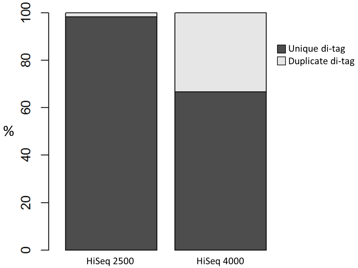
We recently used a HiSeq 4000 and a HiSeq 2500 – which uses a conventional flow cell – to sequence the same Hi-C library. (Hi-C is a technique used to determine the three-dimensional conformation of a genome. This is achieved by performing paired-end sequencing of Hi-C di-tags, which comprise two DNA fragments ligated together. These fragments derive from different genomic positions that were in spatial proximity in the nucleus (Lieberman-Aiden et al.).) The sequencing data were processed using HiCUP, a pipeline tailored for mapping and removing artefacts from Hi-C FASTQ files (Wingett et al.). As expected, the HiSeq 4000 generated far more raw reads (383M) than the HiSeq 2500 (257M). Surprisingly however, the proportion of duplicates differed substantially between the two sequencing runs of the same library. Only 2% of the HiSeq 2500 di-tags were removed after de-duplicating, in stark contrast to the 33% removed from the data generated by the HiSeq 4000. The effect of duplicate removal was to leave both samples with 55M reads at the end of the HiCUP pipeline, thereby offsetting the initial gain made by the increased read output of the HiSeq 4000.
Diagnosis
Before investigating the differences between the two machines, we wanted to rule out the possibility that the increased proportion of duplicates detected by the HiSeq 4000 was simply a result of sequencing more di-tags – i.e. the more a sample was sequenced the higher the probability that any given read was a duplicate. To check for this, the HiSeq 4000 FASTQ file was randomly downsized to the same number of reads as found in the file generated by the HiSeq 2500. During HiCUP processing 25% of the di-tags were now discarded during the de-duplication step, still far more than the 2% discarded than when processing the HiSeq 2500 data.
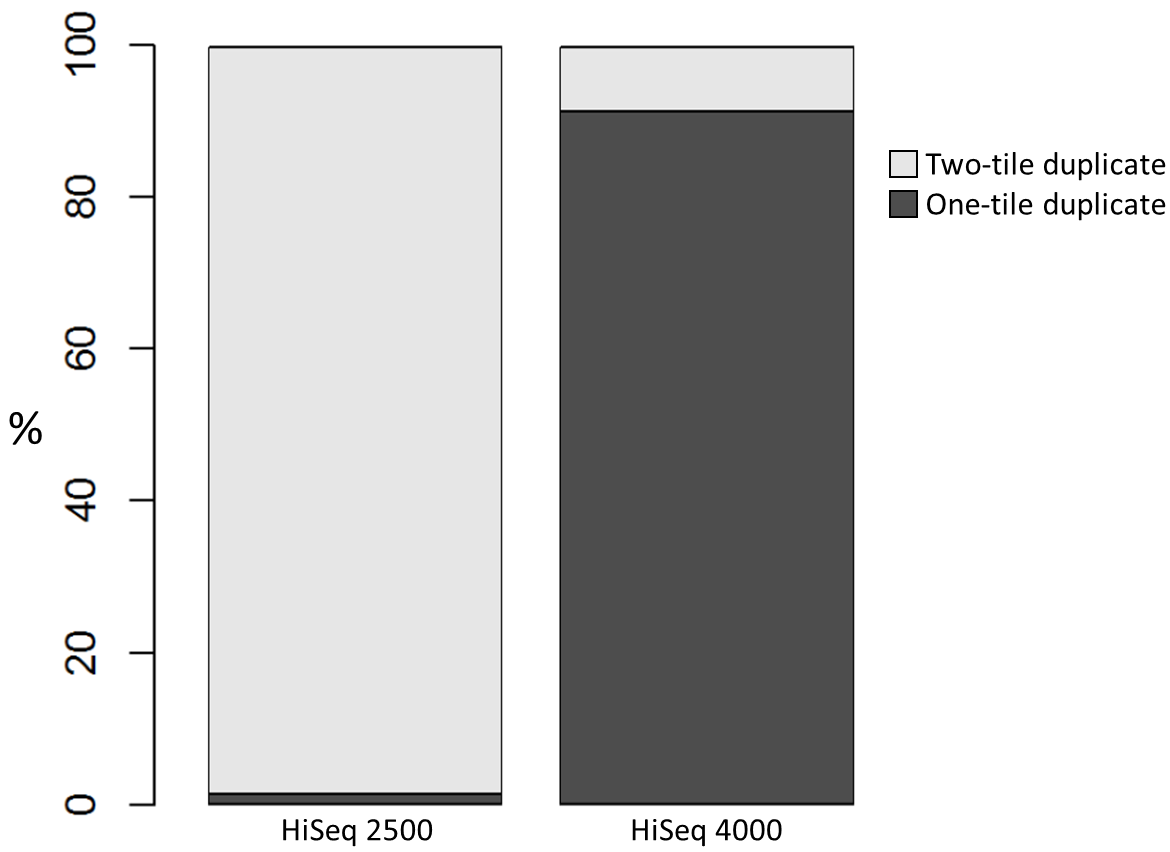
To investigate the possible cause of the duplication we analysed the spatial distribution of duplicate di-tags on the flow cells. For both machines the duplicates were scattered in a uniform manner and did not show significant duplication “hotspots”. While duplicates were not localised to particular regions of a flow cell, it was still possible that, in general, duplicate di-tags may have co-localised with their exact copies. To test this hypothesis we identified di-tags present in two copies and recorded whether they mapped to one or two tiles (each Illumina flow cell comprises multiple tiles). Significantly, 1% of HiSeq 2500 duplicates comprised di-tags originating from the same tile. In contrast, 92% of the duplicate pairs were located on a single tile for the HiSeq 4000. This close proximity suggest that the duplicates observed on the HiSeq 4000 were largely machine-specific artefacts.
To further characterise this two-dimensional separation, we extracted duplicates which localised to only one tile and then recorded the relative position of a di-tag to its exact duplicate (this is possible because FASTQ files record the coordinates of each cluster). The figures below show these findings as density plots (for each di-tag, one read was specified as the origin, and the chart shows the relative position of the “other ends” to the origin).
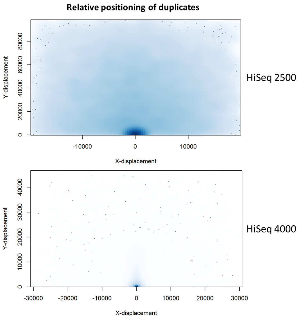
For the HiSeq 2500 there is, in general, a uniform distribution across the plot, except for a high-density region in close proximity to the origin. This elevated density around the origin is much more pronounced when analysing the HiSeq 4000 data, in which almost all the other-ends localise to this region. We hypothesise that the other-ends positioned far alway from the origin are true biological duplicates or experimental PCR duplicates. In contrast, those other-ends close to the origin are more likely to be generated by the machine itself. Again, this is indicative of the HiSeq 4000 generating more duplication artefacts.
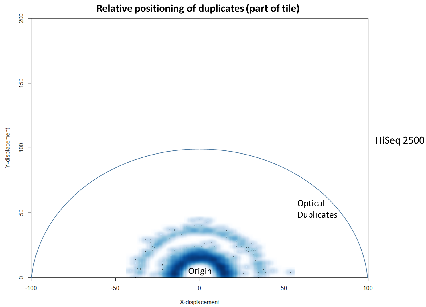
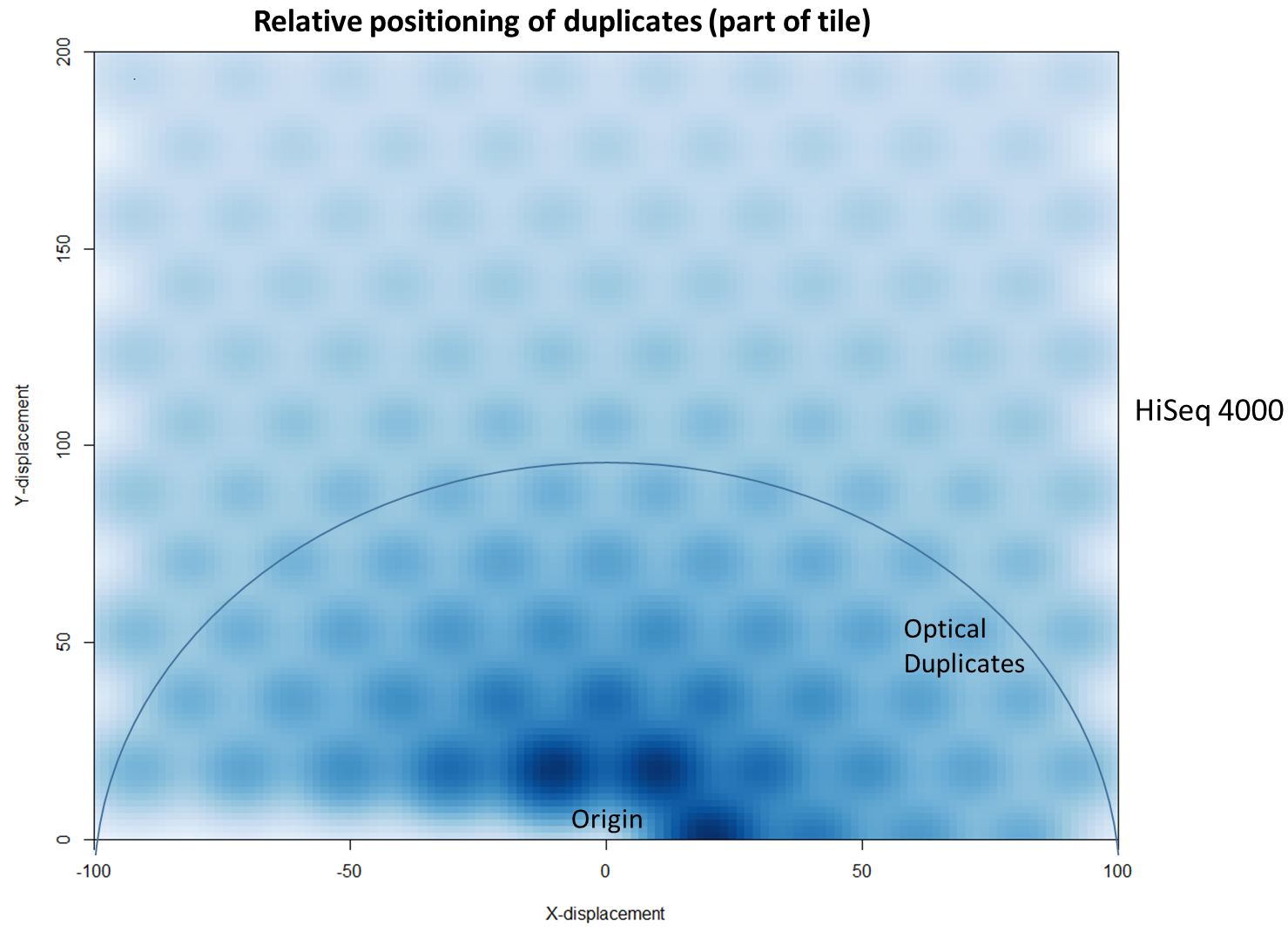
We then investigated whether such duplicates on the HiSeq 4000 were confined to adjacent nanowells, or multiple nanowells in the same local region of a flow cell. Although we were unable to obtain direct information relating the FASTQ coordinate system to individual nanowells, it was possible, by creating a density plot of the region immediately around the origin, to visualise the ordered array of the HiSeq 4000 flow cell. The plot clearly shows that duplicates are found in multiple wells around the origin, and this trend decreases as one moves from the origin. Also shown below is the same plot, but of the HiSeq 2500 data. As expected no nanowell pattern is visible.
Mitigation
Considering the vast potential combination of Hi-C interactions, it should be expected a priori that exact sequence duplicates are more likely artefacts than independent Hi-C events, which has indeed been shown to be the case (Wingett et al.). (Indeed, sequencing Hi-C libraries presents a good method to quantify levels of experimental duplication.) Consequently, duplicates may be identified and removed as part of a standard Hi-C bioinformatics pipeline. This is important since duplicates which do not reflect an underlying biological trend may not only reduce the potential complexity of a data set, they may lead to incorrect inferences being drawn in the post-sequencing analysis. This is a particular problem if certain DNA molecules are inherently more likely than others to form duplicates. For example, it was suggested to us that DNA fragment length may affect duplication rate (in fact we found no evidence for this on further inspection of the data, but nevertheless the potential problem of duplication bias still stands).
Although it is relatively straight-forward to remove duplicates from a mapped dataset, this is not always desirable when genome coverage is high and exact duplicates should be expected, as often observed in RNA-Seq experiments. With the knowledge that patterned-flow cells produce duplicates which are positioned close together, it should be possible to model the separation of such artefacts and set a “proximity filter” to selectively remove them. The histogram below shows the frequencies of the separation distances between duplicates generated on the HiSeq 4000.
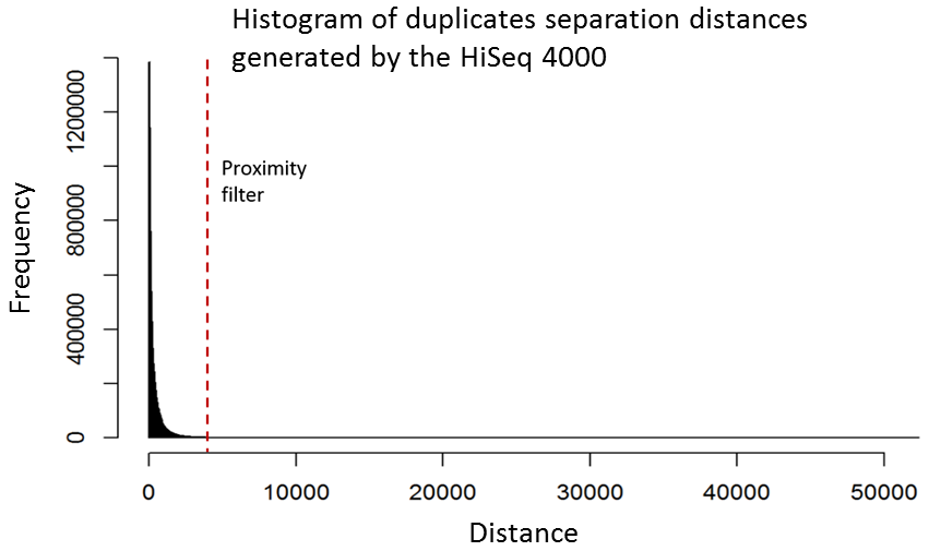
In fact, there are tools already available to identify and label duplicates positioned extremely close together, and these are termed “optical duplicates”. Such duplicates are already known to occur on unpatterned flow cells and result from optical sensor artefacts. Picard is commonly used bioinformatics software than can identify such duplicates. However, by default the program expects duplicates to be within 100 pixels (as illustrated on the density plots above). Although this filter does remove the intense signal around the origin for unordered flowcells, it does not however eliminate ordered flow cell duplicates. In light of this, the Picard documentation recommends increasing the filter to remove duplicates separated by a distance less than 2500 pixels when analysing data generated on a patterned flow cell. This is broadly in agreement with the histogram above and should remove most machine-generated artefacts
While this proximity filtering strategy does mitigate the problem when applied as an “in-house” sequencing/bioinformatics pipeline, it will not be applicable to data submitted to public repositories in which FASTQ header information (which records the cluster co-ordinates) has been removed. Consequently, conclusions reached when processing such third-party data may incorrect owing to duplication biases.
Prevention
The increased propensity for duplicate generation on patterned flow cells has been discussed previously by other researchers. In a recent article published on the CRUK-CI Core Genomics blog, James Hadfield reported that library molecules from a cluster may return to the surrounding solution and then act as a seed for second cluster in a nearby flow cell. It was proposed that these re-seeding events may be minimised by increasing the loading concentration of a library, although this would be at the expense of creating unusable polyclonal clusters. Consequently, a balance would need to be made between these two competing problems to maximise the number of unique valid DNA sequence reads. We discussed this directly with Illumina who agreed with this strategy and suggested that patterned flowcell machines may need to be calibrated on a sequencer-by-sequencer basis to determine optimal loading concentrations.
Lessons Learnt
While patterned flow cells, as seen on the HiSeq 4000, generate a substantially increased number of reads, there is increased scope for duplicate generation. It appears the patterned design of the flow cell, intended to increase discrimination between tightly packed clusters, may itself lead to the generation of duplicates. Such duplicates lead to reduced sequencing depth and the potential to skew experimental results. To ameliorate this situation requires further experimental preparation and possibly sequencer-specific bioinformatics filtering of results.
References
Lieberman-Aiden, Erez et al. “Comprehensive Mapping of Long Range Interactions Reveals Folding Principles of the Human Genome.” Science (New York, N.Y.) 326.5950 (2009): 289–293. PMC. Web. 13 Feb. 2017.
Wingett, Steven et al. “HiCUP: Pipeline for Mapping and Processing Hi-C Data.” F1000Research 4 (2015): 1310. PMC. Web. 13 Feb. 2017.
Software
HiCUP, using defaults but retaining intermediate BAM files that contained putative duplicate di-tags. HiCUP used Bowtie 2 as the sequence aligner.
Picard: Java tools for manipulating sequencing data and formats such as SAM/BAM/CRAM and VCF.
Soft-clipping of reads may add potentially unwanted alignments to repetitive regions
Introduction
Next Generation Sequencing applications can interrogate a wide variety of biologically relevant molecules, events or modifications. Examples could be genome resequencing, RNA-Seq, ChIP-Seq or Bisulfite-Seq, to name but a few. The mapping efficiency (= the total number of reads that align) typically depends on several factors such as i) the technical quality of the reads, ii) the read length, iii) the alignment software used, iv) the absence of contaminants (such as other species or adapter contamination) and last but not least v) the quality of the reference genome assembly. Also the type of the experiment may have an influence, e.g. while RNA-Seq typically aligns back to the genome fairly well, techniques that tend to enrich repetitive sequences or Bisulfite-Sequencing (which only uses a 3-letter alphabet for mapping and often requires unique mapping) typically display somewhat lower mapping efficiencies.
Real life datasets are often not perfect however, they may contain poor basecall qualities, sequencing errors, insertions or deletions relative to the reference genome, unwanted sequences (e.g. contaminants) or read-through adapter contamination where the read length is longer than the sequenced fragment. While adapter/quality trimming and allowing for several mismatches and InDels allows to rescue most of these reads, a still fairly sizeable proportion of reads in the library may consist of sequences that are not present in the genome assembly and as a result cannot be placed at all.
The Symptoms
Despite the limitations of both reads and genome builds there are aligners out there claiming to have placed close to 100% of reads properly. This just sounds a bit to good to be true, so we tried to investigate this in a bit more detail…
Aligners reaching such high mapping efficiencies often perform so called “soft-clipping” of reads. This essentially means that portions of the read that do not match well to the reference genome on either side of the read are ignored for the alignment as such. This procedure carries a small penalty for each soft-clipped base, but it amounts to a significantly smaller alignment penalty than mismatching bases. Some programs even claim that this makes adapter trimming obsolete because as soon as the sequence does not align to the reference any more it will be soft-clipped.
Diagnosis
To get to the bottom of the differences between global, or end-to-end, mapping where the read has to align from the start to the end, and local mapping, where only a part of the read has to map and the ends may be soft-clipped, we decided to use several different library types that had undergone quality and adapter trimming using Trim Galore. This step should reveal the differences between end-to-end and local mapping without being affected by quality and/or adapter issues.
RNA-Seq
We started off by comparing some RNA datasets (single-end, 100bp, mouse genome GRCm38) using Hisat2 which in its current implementation (v2.0.3-beta) performs soft clipping (local, y-axis) by default (even though it is sort of undocumented), and the same dataset run using the option ‘–sp 1000,1000’ which effectively renders soft clipping impossible (end-to-end, EtE, x-axis).
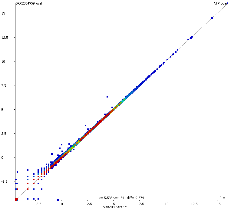
The data (quantified as log2 reads over protein coding transcripts) looked virtually identical between the two options, showing that for RNA-Seq data soft-clipping doesn’t seem to make a noticeable difference for downstream analysis. This is perhaps not surprising because RNA-Seq data represents rather well annotated and not very repetitive regions of the genome.
Genomic DNA
Next we looked at genomic DNA alignments, more specifically some randomly chosen ChIP-Seq or Input samples (either 50 or 100bp, single-end, mouse GRCm38 genome, again trimmed with Trim Galore). For the comparison we used Bowtie2 (v2.2.7) in end-to-end (EtE) or local (–local) mode.
The mapping statistics presented the following picture:
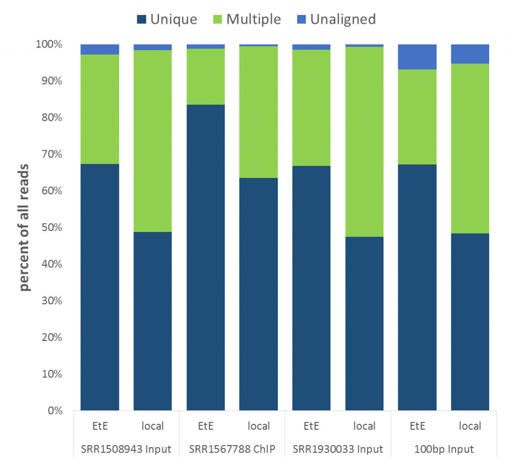
Soft-clipping was able to place more reads that were previously unaligned, but since the fraction of Unaligned reads was rather small to start with the effect didn’t look very dramatic. More striking was that in all data sets analysed the fraction of Unique reads was reduced while ambiguous alignments went up by roughly the same amount. In other words, it appeared as if reads that were previously aligned uniquely were soft-clipped to a shorter length so that they do now align to several places in the genome, i.e. repetitive sequences. As pointed out above we did not see this effect for the RNA-Seq data probably because it doesn’t contain as many repetitive sequences as applications using genomic DNA.
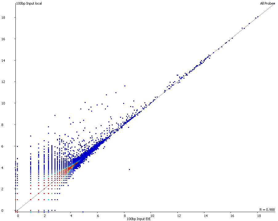
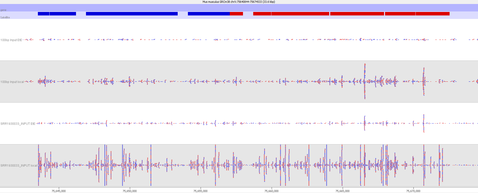
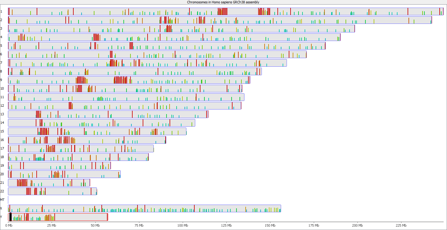
A scatter plot of end-to-end (x-axis) and local (y-axis) showed quite a number of regions with much increased read counts in local mapping (reads were quantified over 2kb genomic regions using log2 counts). When visualised on a genome-wide scale the regions with high read counts exclusively with local alignments accumulated suspiciously close to chromosome ends or other gaps in the genome assembly, suggestive of centromeric or telomeric repeats.
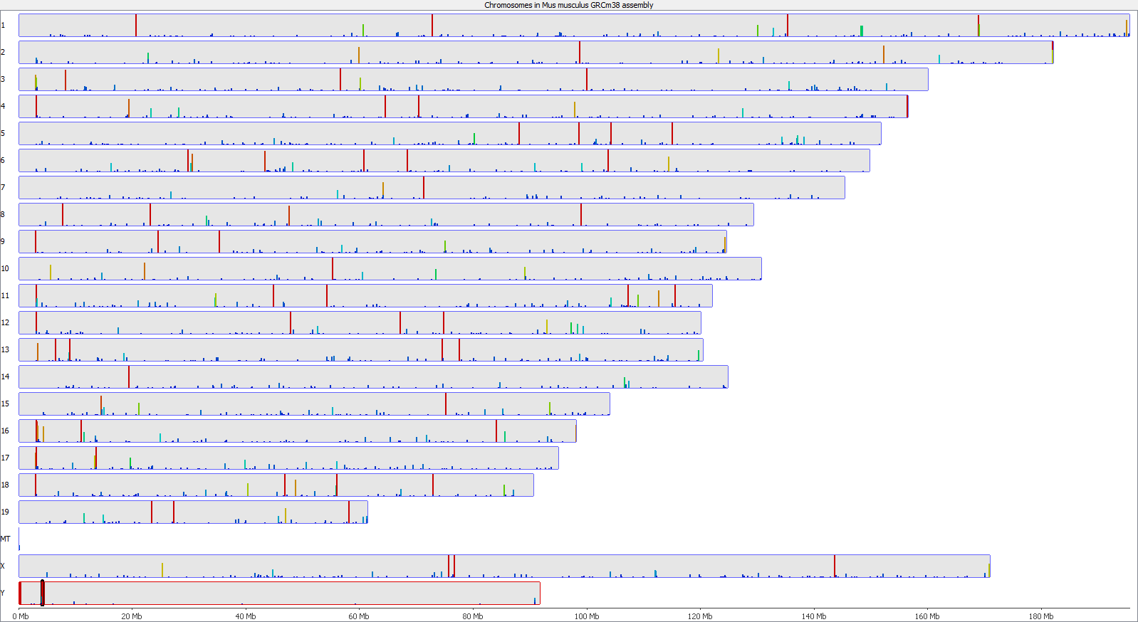
Indeed we found that a large proportion of regions (>80%) with high read counts overlapped annotated Satellite repeat regions (RepeatMasker), such as this one:
Bisulfite-Seq
Lastly we also wanted to take a look at Bisulfite-Seq (BS-Seq) because it is special for a few reasons:
- many aligners in-silico convert C to T in both reads and the reference genome during the mapping; this 3-letter alphabet approach makes it more difficult to place alignments uniquely
- most bisulfite aligners require unique alignments because it is not ‘safe’ to call methylation states if you can’t be sure where a read really came from
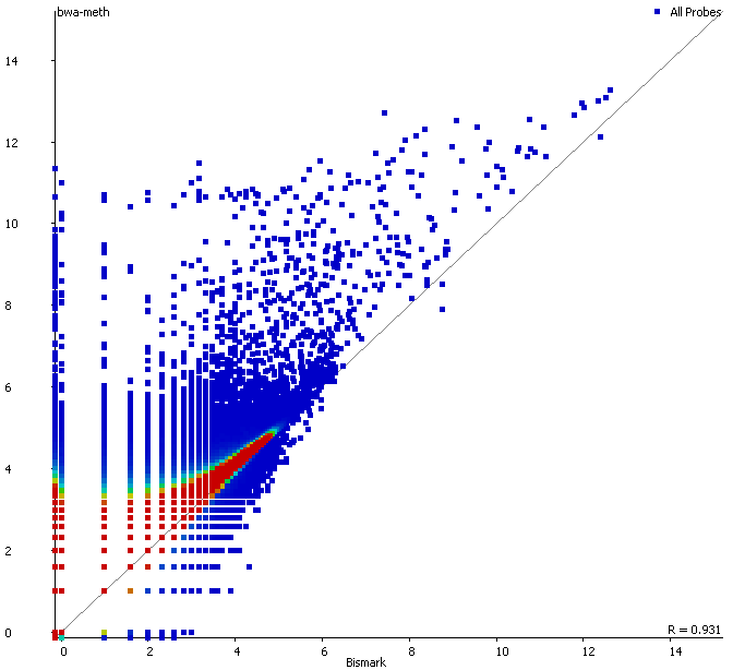
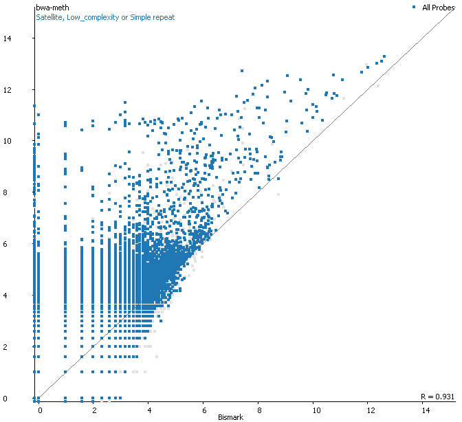
Because of these ‘features’ it is difficult to exceed alignment efficiencies of ~86% for human or ~78% for mouse for typical BS-Seq experiments (with say 100bp reads), yet soft-clipping still achieves alignment rates of 95-100% also in this setting. To look at differences between end-to-end mapping and soft clipping in a BS-Seq library we used 125bp human reads (trimmed with Trim Galore) in single-end mode against GRCh38 (plus decoys), and used Bismark (end-to-end) and bwa-meth (soft-clipping) as examples.
First of all it is good to see that the two methods generate virtually identical results for the vast majority of the genome as can be seen here (soft-clipping top, end-to-end bottom):
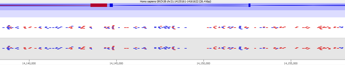
There are however also regions showing drastic differences in read depth (2kb tiled windows, log2 counts):
Regions with increased counts in the soft-clipped data do again cluster mainly towards ends of chromosomes or regions that have large gaps (or Ns) in the genome build.
Filtering for overlaps with Satellite, Low Complexity or Simple Repeat regions for the human genome (RepeatMasker) explains nearly all of the coverage differences:
Here is a browser shot of one these regions illustrating the differences in read coverage (soft-clipping top, end-to-end bottom):
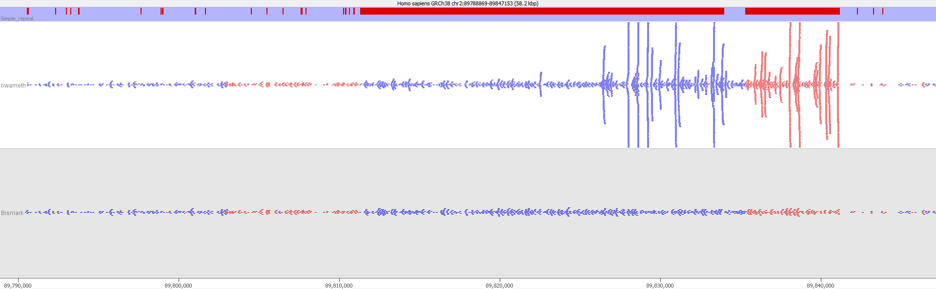
What happens in these cases is that reads which do not align anywhere in the genome (probably because they are not actually present in the genome build) are soft-clipped until a part of the read can be placed somewhere – unfortunately this newly ‘gained’ mapping position is not necessarily the correct one. While it might be informative to know that some part of a read resembles a certain type of repeat it is the wrong thing to place a read uniquely to a near-enough partial match of the sequence, and in case of bisulfite data then infer the region’s methylation state from such alignments.
Mitigation and Prevention
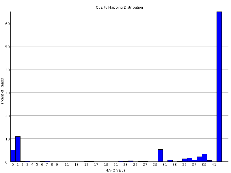
Luckily such hot-spots where soft-clipped reads get assigned incorrectly to repetitive regions in the genome can easily be spotted by their coverage, which tends to be hugely higher than for the rest of the genome. These reads could be removed by virtue of the abnormal coverage, but they are better handled by filtering on the read MAPQ values:
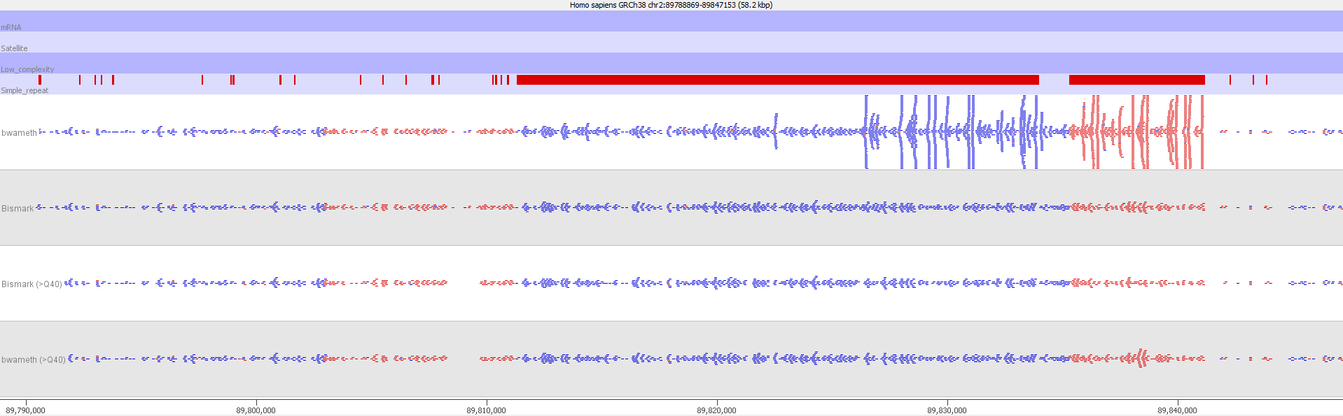
Filtering out reads with a MAPQ of <40 effectively removed all of the dodgy alignments, rendering the results virtually indistinguishable from end-to-end alignments again.
Lessons Learnt
The take home message from this is that soft-clipping of reads may force reads to align somewhere in the genome even if the location is not the true origin of reads, and this is most apparent for repetitive regions of the genome. This doesn’t mean that soft-clipping per-se is a bad thing, in some cases it might rescue some true alignments e.g. from technical problems such as the overcalling of Gs on the NextSeq platform (until it has been properly addressed by Illumina), or for the detection of structural variations in the genome.
For standard genomic alignments however we believe that it is important to understand the data at hand, know which kind of contamination may occur at the read ends (e.g. adapter sequence) and remove those and poor qualities accordingly. And one has to be aware that ‘magically’ increasing the mapping efficiency to close to 100% comes at the cost of potentially including a ton of incorrect alignments with all the side effects this may have on downstream analysis (e.g. correction, statistical power etc.)
Illumina 2 colour chemistry can overcall high confidence G bases
Introduction
Illumina sequencing chemistry works by tagging a growing DNA strand with a labelled base to indicate the last nucleotide which was added. 4 different dyes are used for the 4 different bases and imaging the flowcell after each base addition allows the machine to read the most recently added base for each cluster.
In the standard version of this system used on HiSeq and MiSeq instruments each cycle of chemistry is followed by the acquisition of 4 images of the flowcell, using filters for each of the 4 emission wavelenths of the dyes used. The time taken for this imaging is significant in the overall run time, so it would obviously be beneficial to reduce this.
With the introduction of the NextSeq system Illumina introduced a new imaging system which reduced the number of images per cycle from 4 to 2. They did this by using filters which could allow the simultaneous measurement of 2 of the 4 dyes used. By combining the data from these two images they could work out the appropriate base to call.
4 colour detection
| Base | G filter | A filter | T filter | C filter |
|---|---|---|---|---|
| G | Yes | No | No | No |
| A | No | Yes | No | No |
| T | No | No | Yes | No |
| C | No | No | No | Yes |
2 colour detection
| Base | A+C filter | T+C filter |
|---|---|---|
| G | No | No |
| A | Yes | No |
| T | No | Yes |
| C | Yes | Yes |
The problem here though is that there is a fifth base option, which is that there is no signal there to detect. This could happen for a number of reasons:
- There is no priming site for this read, so no extension is happening. If this happens in the first read then it just won’t detect a cluster, but in subsequent reads the cluster will be assumed to still be present.
- Enough of the cluster has degraded or stalled that the signal remaining is too faint to detect
- Something is physically blocking the imaging of the flowcell (air bubbles, dirt on the surface etc etc)
In the 4 colour system this extra option is easy to identify since you get no signal from anything, but in the 2 colour system we have a problem, since no signal in either channel is what you’d expect from a G base, so you can’t distinguish no signal from G.
What we find therefore on Illumina systems running this chemistry is that we see an over-calling of G bases in these cases, and this can cause problems in downstream processing of data.
The Symptoms
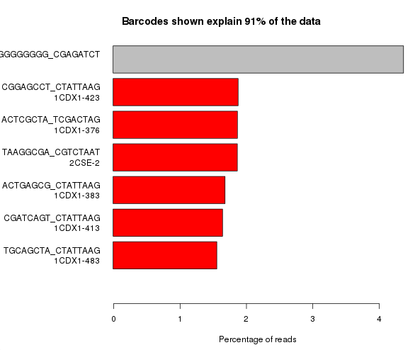
There are a couple of different ways in which this problem can manifest itself. Possibly the most obvious is that you can get a huge over-representation of poly-G sequences in reads other than the first read (which is used for cluster detection). From reports we’ve seen this seems to be most prevalent in the first barcode read, but could presumably affect any read where the initial priming of the read failed for any reason.
The example below is the top of a barcode splitting report for a sample which had a lot of barcodes. You can see that the most frequently observed barcode for this sample had polyG for barcode1, and that this wasn’t expected. You can also see that the second barcode was read correctly so the cluster itself was OK, but for some reason just didn’t prime for the barcode 1 read.
If we extract out the polyG sequences from the first barcode read and look at their quality distribution we see that the qualities are universally high, so there’s no way to distinguish these mis-calls by using the normal quality control mechanism.
This then leads to the second type of problem seen in these datasets. This occurs when the signal from a cluster completely degrades. In a 4 colour system this would result in a somewhat random base call, but a very low quality score to reflect the low level of signal. In a 2 colour system the quality will initially fall as the signal degrades, but eventually the signal will effectively disappear and the sequencer will start calling high quality G bases.
The sequence below shows this effect:
@1:11101:2930:2211 1:N:0
ATTTATTATTAATTAAATATTAATAATAAATAGATCGGAAGAGCACACGTCTGAACTCCAGTCACTAGCTTAGCGCGTATGCCGTCGTCGGCGTGCAAAAAAAAAGGGGGGGGGGGGGGGGGGGGGGGGGGGGGGGGGGGGGGGGGGG
+AAAAAEEEEEEEEEEEE6EEEEEAEEEEEEEEEA/EE<EEEAEE/EAEEAEEEE6</EEEEEA/<//<///A/A//////</E<//////E///A/</A/<<A////A/E<EEEEEEEAEEE/EEEAEAEAEAE6/AEAEE<AAEAEE
It’s easier to see if you visualise the quality scores for this sequence
You can see that the quality degrades as expected initially, but then the signal disappears, either because of an extension of the general degradation or because some external factor blocked the imaging, and the sequencer starts to call G bases, the quality rises again.
The big issue this cases is that most trimming systems assume that quality loss is progressive from the 5′ end of a read to the 3′, so when deciding where to quality trim a read they start at the 3′ end and work back towards the 5′ until good quality sequence is detected. In the types of read shown above the read will not be trimmed because the most 3′ sequence is high quality, so incorrect base calls will remain which will adversely affect the downstream analysis of this data.
Mitigation and Prevention
There are a few potential strategies for fixing this problem and some of the symptoms will be easier than others. For unprimed reads which are completely polyG then these will probably not affect downstream analyses other than triggering QC alerts, so will have less of an impact once people are aware of their source. For the progressive quality loss the need for a solution is more pressing. Illumina already have a system in place which artificially downweights the quality scores for reads whose quality dips below a certain level. It seems likely that they should be able to adapt their calling software to recognise reads where quality dips to be replaced with high quality poly-G and then artificially downweight the quality scores for the remainder of the read. This same case can probably also be tacked by the authors of trimming programs where they might, for example, provide and option to exempt G calls from the assessment of quality and to trim 3′ Gs from reads as a matter of course.
Lessons Learnt
You can’t always trust the quality scores coming from sequencers, and if you see odd sequences in your libraries it’s worth investigating them as they may unearth a deeper problem.
Acknowledgements
Many thanks to Hemant Kelkar, Marcela Davila Lopez, Stuart Levine and Frederick Tan for their help in understanding this issue.
Mixing sample types in a flowcell lane generates cross contamination artefacts
Introduction
A single lane on an Illumina sequencer can generate in excess of 200 million reads – far in excess of what is needed for many common sequencing applications. It is therefore common to put multiple samples in the same lane, and to use barcode sequences to be able to determine the original source for each read so you can separate them later on.
The most common use of barcoding is to mix together multiple samples from the same experiment, where all of the samples will be of the same type and from the same species, but we have frequently seen cases where people want to mix very different libraries together. Whilst we have strongly recommended against this for a long time (and don’t even allow samples to be annotated that way in our LIMS), people persist in doing this so it seemed worthwhile illustrating why this is a bad idea.
The root problem here is that barcoding is not a foolproof technology. Even with stringent separation criteria (all barcodes must be read exactly correctly over their entire length), you will still get a small amount of cross contamination between the libraries within a single lane. Whilst this will be a randomly selected subset of reads and will represent only a fraction of a percent of the total data, this can still have a devastating effect on the analysis of some library types and is very difficult to fix retrospectively.
The Symptoms
This issue is well illustrated in by the following genome view of two ChIP-Seq lanes which are ChIPing for the same factor.
On the face of it it looks like the top sample has a number of extra peaks which would appear to be novel binding events. A closer examination however makes these novel peaks appear somewhat suspicious. In particular you can see that the novel peaks are directional (red = top strand, blue = bottom strand), whereas ChIP peaks would normally not be expected to exhibit any directionality.
If we look more closely at one of the peaks then things get more suspicious.
Now we look more closely it becomes very obvious that this is an issue of contamination. The extra peaks sit within the exons of transcripts and their directionality is always opposite to the direction of the feature. Our suspicion therefore would be that this ChIP sample has become contaminated with a reverse strand specific RNA-Seq library. Looking at the sequencer annotation we find that this is exactly what has happened – the user had mixed ChIP and RNA-Seq samples in the same lane and even though the libraries hadn’t seen each other until they were mixed within the flowcell, we still see this mis-annotation of reads.
The level of cross contamination seen here is very high compared to what you’d normally expect, but in this case it was exacerbated by a secondary effect – this was a highly duplicated library, so the user had deduplicated their data. The deduplication had removed a large proportion of the ChIP library, but the contaminating RNA-Seq data was not duplicated and wasn’t affected by the deduplication – amplifying the effect of the contamination. The same sort of effect will happen in other libraries though but may not be as obviously visible.
Mitigation
There is no way to completely prevent mis-annotation of barcoded reads in a sample. There are enough cases where you see a perfect, but incorrect, barcode that there’s nothing you can do to remove these. This may be an optical issue (mismatching the reads from barcodes and inserts), or some kind of internal recombination the flowcell, but really the exact source doesn’t matter for the purposes of this article.
The mitigation here is to make sure that the way you mix your libraries together will mean that it won’t matter if a very small percent of reads leak from one library to another. Generally this means keeping the same library type in the same lane.
If you have two similar libraries (genomic libraries for example) in the same lane and a tiny proportion of crossover occurs then since the overall distribution of reads between the two libraries is likely to be similar the proportional effect on any given position within the libraries will be negligible. However if your libraries have strong biases in their composition (RNA-Seq for example) then a random selection of reads from these will not be randomly distributed over the genome. A highly expressed gene in RNA-Seq could potentially have millions of reads over it, so that tens or hundreds of these reads could end up cross contaminating other libraries, making it look like something interesting was happening at this position.
To illustrate this I took a pretty normal RNA-Seq library with ~20million reads in it and randomly select 2000 reads from it (that’s around 0.01% of the data – easily within the range of mis-annotated reads). You can see that the reads are not uniformly distributed over the whole genome but preferentially fall within a few regions which relate to the most highly expressed genes.
Looking in more detail at a single locus you can see that although the absolute number of reads is not enormous, if these were overlaid on a flat background they would appear to be a significant local enrichment. For enrichment seeking library types such as ChIP this could easily be misinterpreted, and if you were looking for rare events in a SNP detection or something sensitive such as a Hi-C experiment then this could appear to be a hugely enriched signal.
Lessons Learnt
Sequencers aren’t perfectly clean in their ability to separate barcode mixes put into them. You can minimise the effect of cross-contamination by only mixing samples from within the same experiment, but even then you might want to consider whether your results could be biased by the addition of a small number of randomly selected reads from another library in the same lane.
Genomic sequence not in the genome assembly creates mapping artefacts
Introduction
In many ways mapping of sequence reads to a reference genome is a solved problem. If we know the sequence of the underlying genome and have a good error model for the data generated by the sequencing platform then we can show that it’s possible to assign the most likely mapping position for a read, and to associate this with a meaningful p-value for the likelihood that the reported position is, in fact, correct.
This rosy picture can become muddied somewhat though. A simplistic mathematical view of mapping starts from the assumption that we have perfect knowledge of the reference genome, and in practice that’s not true. Even where we have very mature genome assemblies for human / mouse etc there are still relatively large regions of the genome where the exact sequence is not known. Mainly these regions consist of long stretches of highly repetitive sequence which is almost impossible to position accurately with current sequencing technologies. In some cases these regions may even be variable between different individuals or cells so there is no true reference. Examples of these types of regions would be telomeres, centromeres and satellite sequences, but other smaller repetitive regions will also suffer the same problem.
These problematic repetitive regions will still generate reads in an experiment and these cause trouble for the read mappers. Because the true mapped position for these reads isn’t shown in the assembly the read mappers can end up mis-judging the likelihood of the next best position they find as being correct, leading to these reads being incorporated into the data used for downstream analyses.
The figure below shows a simplified view of the problem.
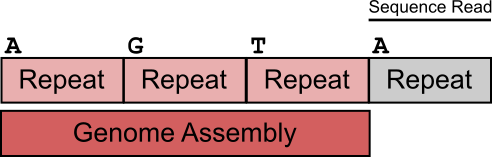
In this example we have a stretch of repeats with a minor variation in their first base. 3 of the repeats are within the genome assembly, but the last one was not assembled and doesn’t appear in the reference. If a read comes from this last repeat the correct mapping answer would be to map it to either the first or last copies of the repeat (which contain an A), but to flag it as a non-unique alignment. Since the read mapper can’t see the last repeat in the reference though the read will incorrectly be mapped to the first repeat, and will be listed as a unique alignment, since this is how it appears.
The Symptoms
These types of mis-mapping occur in all library types, but are very easy to spot when you have a library which should produce even coverage over the whole genome. The example below is a genomic library which is showing only reads reported to be a unique best alignment against the genome and you can clearly see a number of very high coverage peaks where mismapped reads have accumulated.
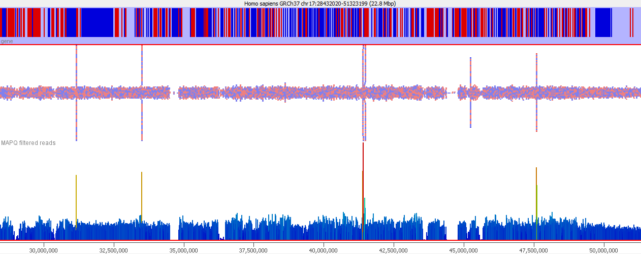
Looking on a wider scale you can see that these peaks often occur at the edges of holes in the genome. This is because these regions tend to be enriched for the class of repeats which fill the hole in the genome, so mis-mappings tend to accumulate there.
It’s probably also worth pointing out that although this issue is most obvious in the largest classes of repeats, it will also affect the majority of repeat classes to a lesser degree, and could even affect repetitive gene families.
Mitigation and Prevention
There are two approaches to dealing with these types of reads.
- You can try to identify the places in the genome where the mis-mapped reads accumulate and mask these from any analysis you’re doing as being unreliable.
- You can try to adjust the way you do your mapping to prevent the erroneous mapping in the first place.
Filtering coverage outliers
Identifying regions which accumulate mis-mapped regions is relatively simple in library types where even genomic coverage is expected. You can use standard methods for outlier detection to find places in the genome which have a statistically unlikely density of reads. Most of these regions have coverage levels several orders of magnitude above the background so fairly stringent cutoffs can be used to avoid losing other regions with more marginal enrichment for other reasons.
If however you are working within a library type where enrichment is expected (ChIP-Seq for example) then this type of approach may not be practical. Because the mis-mappings are characterised by the genome assembly and mapper used though, you can transfer the set of positions you have learned on another dataset (or on the input for the ChIP) and use these to mask the enriched data.
For some genomes there are published lists of blacklisted regions assembled from large genome sequencing projects which can be used as annotation tracks to filter your data or results and to save you from having to define problematic regions in your own data. These predictions can be an easy shortcut to use if you work in one of the genome assemblies they support.
Improving read mapping
The other approach to take to fixing this problem (which can be used in concert with the above filtering), is to try to get more accurate mapping in the first place. The root of this problem is that some regions which are in the genome are excluded from the assembly and are therefore invisible to the mapping programs.
In some cases the missing regions are present in shorter assembly contigs which are part of the original draft assembly but are not able to be placed into the scaffolded chromosomes. These additional contigs are sometimes distributed with the genome sequences, but excluded from analysis. Leaving such short contigs in place during mapping will improve the mapping statistics, even if those contigs aren’t actually analysed in the downstream pipeline.
Another approach is to try to construct artificial sequences containing the missing sequences in an unstructured format. These ‘read sinks’ or ‘sponge databases’ aren’t intended to generate data to analyse directly but provide enough context sequence for the read mappers to correctly interpret the correctness of mapping for repetitive reads.
References
PBAT and single-cell (scBS-Seq) libraries may generate chimeric read pairs
Introduction
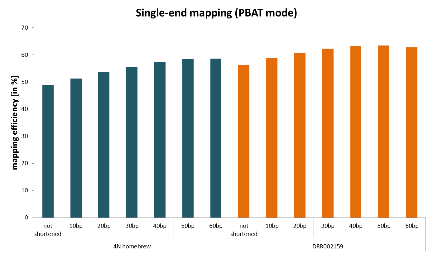
Shortly after the initial PBAT publication (which was single-end data), people started to optimise the protocol for extremely low starting material. We quickly noticed that the mapping efficiency for paired-end experiments (4N random priming initially) was rather low. We’re aware of adapter contamination and poor quality basecall issues, and more recently learned about mispriming biases in PBAT, but still the alignment efficiencies we observed were sometimes much lower than what we would expect despite rigorous adapter and quality trimming (we are talking about anything between ~30-50% for 2x100bp libraries).
The Symptoms
We then sought to identify why the mapping efficiencies were so low by hard-trimming single-end reads by a further 10, 20, 30 etc. basepairs from their 3′ end after adapter/quality trimming and removing the first biased 4bp (see here) with Trim Galore. We found that shortening the reads more and more resulted in ever increasing alignment rates despite the fact that really short bisulfite reads are significantly more difficult to align due to increasing the chances of multimapping reads because of the reduced search alphabet during bisulfite mapping (only G, A and T). This was not limited to our home-brew PBAT protocol but was also true for the originally published (single-end) data.
This indicated that something must have been present in the reads that prevented them from mapping efficiently.
Diagnosis
We reasoned that the sequenced fragments might be crossovers of different genomic sequences that were somehow generated during the two steps of random priming and strand extension. To test whether such chimeric reads really existed we aligned Read 1 and Read 2 of our paired-end library individually and teamed the aligned reads up by their read ID in a post-processing step.
The data was then imported into SeqMonk as a Hi-C input BAM file so that we could keep track to of what partner reads were doing. Shown below is a quantitation of all partner reads where the first end aligned to chromosome 1 (red = high number of partner reads, blue = low number of partner reads). This showed that the majority of Read 2 partners also aligned to chromosome 1, presumably most as valid paired-end alignments.
Strikingly however this also showed that there was an appreciable fraction of trans-hits, i.e. reads with Read 1 on chromosome 1 and Read 2 on a different chromosome. Even though there were a few hotspots (red bars) the interacting reads appeared to be spread out more or less evenly over the entire genome, so it was not just say a single type of repetitive element that preferentially formed read chimaeras. The number of trans-reads in the sample examined accounted for nearly 30% of all read pairs, so this is can be substantial problem.
Edit March 2019 for single-cell bisulfite sequencing (scBS-seq):
A recent article in Bioinformatics (https://www.ncbi.nlm.nih.gov/pubmed/30859188) also demonstrated in that chimeric reads are also the main problem for the low mapping efficiency in scBS-seq. In their article, Wu and colleagues demonstrate that the post-bisulfite based library construction protocol leads to a substantial amount of chimeric molecules as a result of recombination of genomic proximal sequences with ‘microhomology regions (MR)’. As a means to combat this problem the authors suggest a method that uses local alignments of reads that do not align in a traditional manner, and in addition remove MR sequences from these local alignments as they can introduce noise into the methylation data.
Mitigation
Such chimeric “Hi-C like bisulfite reads” deliberately do not produce valid (i.e. concordant) paired-end alignments with Bismark. To rescue as much data from a paired-end PBAT library with low mapping efficiency as possible we sometimes perform the following method (affectionately termed “Dirty Harry” because it is not the most straight forward or cleanest approach):
- Paired-end alignments (
--pbat) to start while writing out the unmapped R1 and R2 reads using the option--unmapped. Properly aligned PE reads should be methylation extracted while counting overlapping reads only once (which is the default). Also mind 5′ trimming mentioned in this post. - unmapped R1 is then mapped in single-end mode (
--pbat) - unmapped R2 is then mapped in single-end mode (in default = directional mode).
Single-end aligned R1 and R2 can then be methylation extracted normally as they should in theory map to different places in the genome anyway so don’t require attention to overlapping reads. Finally, the methylation calls from the PE and SE alignments can merged together before proceeding to the bismark2bedGraph or further downstream steps.
Edit March 2019: Please also see above the suggested mitigation approach for scBS-seq data using local alignments.
Prevention
Unfortunately the generation of chimeric reads seems to be inherent to the PBAT library preparation protocol and as such it is not very likely to just go away unless the random priming and extension steps could be optimised somehow. Even though a little cumbersome we found that using the PE alignments first and SE alignments afterwards approach achieves overall alignment rates that are almost in the range observed for whole genome shotgun BS-Seq. As a side note, even though the EpiGnome kit from Epicentre (an Illumina company) uses a PBAT-type amplification protocol it doesn’t seem to be affected very much by chimeric reads which is probably owed to their proprietary way of performing the pulldown/amplification step (which also generates directional and not PBAT libraries…). (Edit: The TruSeq DNA Methylation Kit is now discontinued).
Lessons Learnt
In addition to standard factors that affect most types of libraries (adapter contamination and basecall issues) and mis-priming errors at the 5′ end of reads, PBAT libraries may contain a substantial number of chimeric reads that prevent paired-end reads from aligning as concordant read pairs.
Datasets
Some datasets processed with the method described here may be found here under the GEO accession GSE63417.
Software
Data processing of public or homebrew PBAT data was carried out using Trim Galore and Bismark. Teaming up paired-reads was achieved using a custom written script. Visualisation of “Hi-C like” bisulfite read pairs was done in SeqMonk.
Using local alignment to enhance single-cell bisulfite sequencing data efficiency. Wu P, Gao Y, Guo W, Zhu P., Bioinformatics. 2019 Feb 19. pii: btz125. doi: 10.1093/bioinformatics/btz125. PMID: 30859188
MAPQ values are really useful but their implementation is a mess
Introduction
In various stages of the processing of an NGS dataset it can be useful to filter the data to remove poor quality reads. At an early stage this could be reads with poor quality base calls, but after mapping to a reference genome you may want to filter out alignments which show a poor match to the reference, or which could have mapped to a number of different places in the genome. These ambiguously mapped reads can add a lot of noise to an analysis and will tend to accumulate over repetitive regions. In the example below you can see the comparison of the reads from a standard bowtie2 mapping of a genomic dataset, and the result of applying a MAPQ filter to the data. The peaks over repetitive elements are largely suppressed in the filtered data.
To aid with this task the SAM format specification defines the mapping quality (MAPQ) value. In the spec the value is described as:
MAPping Quality. It equals -10 log10 Pr {mapping position is wrong}, rounded to the nearest integer. A value 255 indicates that the mapping quality is not available.
So in the spec this is pretty clear, it’s analogous to a Phred score in a fastq file in that it’s a simple transformation of the probability that the mapped position reported is wrong.
In practice, unfortunately, the use of this value is much less clear. For many types of read mapper there is no sensible way to put a p-value on the likelihood that a reported mapped position is wrong so rather than stick to the published spec the aligners have taken the valid value range (0-255) and implemented their own scoring scheme on top of this.
In many cases the values encoded in the MAPQ value hold useful information about the reads and are a valuable resource when filtering data, but the variability with which the value is calculated means that it can be difficult to create pipelines which use this value and which are robust to changes in the aligner used.
Implementation
To try to make more sense of this we’ve gone through the documentation of a bunch of the most popular aligners to see how they make use of the MAPQ value.
Bowtie1
Bowtie1 sets the MAPQ value to 255 for uniquely mapped reads and 0 for multiply mapped reads, unless the --mapq flag was added when the program was launched, in which case the value specified will be used instead.
Bowtie2
Reference – this page has a great explanation for how alignments in bowtie2 are scored and MAPQ values are assigned.
Bowtie 2 uses a system of flag values for its mapped alignments based on the number of mismatches of various qualities, and the number of multi-mapping reads.
MAPQ >= X   #MM Q40   #MM Q20      #MM Q0    Description
0           5         7            15        All mappable reads
1           3         5            10        True multi w/ "good" AS, maxi of MAPQ >= 1
2           3         5            10        No true multi, maxi of MAPQ >= 2
3           3         5            10        No true multi,  maxi of MAPQ >= 3
8           2         4            8         No true multi, maxi of MAPQ >= 8
23          2         3            7         No true multi, maxi of MAPQ >= 23
30          1         2            4         No true multi, maxi of MAPQ >= 30
39          1         2            4         No true multi, maxi of MAPQ == 39*
40          1         2            4         No true multi, only true uni-reads
42          0         1            2         Only "perfect" true unireads
In the case of bowtie2 therefore you could use a MAPQ filter of >=40 to get reads which had only 1 convincing alignment, or a lower filter to allow multi-mapped reads where there was a secondary alignment with varying degrees of difference to the primary.
Bismark
The MAPQ values reported in Bowtie1 mode are always 255 (multiply aligning hits are not reported). In Bowtie 2 mode the MAPQ scores are re-calculated using the Bowtie2 scoring scheme.
BWA
BWA actually follows the SAM spec and reports Phred scores as MAPQ values. The calculation is based on the number of optimal (best) alignments found, as well as the number of sub-optimal alignments combined with the Phred scores of the bases which differ between the optimal and sub-optimal alignments.
Tophat
Tophat uses flag values with specific meanings to populate the MAPQ value field. Older versions of tophat set all values to 255 (not available) but any recent version has used an updated scoring scheme.
- 50 = Uniquely mapping
- 3 = Maps to 2 locations in the target
- 2 = Maps to 3 locations in the target
- 1 = Maps to 4-9 locations in the target
- 0 = Maps to 10 or more locations in the target
There are however some caveats which come with these values!
- Tophat has the option to restrict reporting of hits using the -g parameter and unfortunately the calculation of MAPQ values appears to happen after this filtering resulting in all hits being given a MAPQ of 50. This means that to see meaningful MAPQ values you have to set -g to at least 2 (you can then later filter on the primary alignment flag to remove the secondary alignments).
- Tophat uses a dual mapping strategy where it first tries to align to a transcriptome and only if it doesn’t get a good hit there will it search the entire genome. When you have a read which is uniquely mapped within the transcriptome, but has multiple hits within the genome as a whole the hit will be reported as unique and given a MAPQ of 50, which can result in artefacts in downstream analyses.
STAR
Star uses a similar scoring scheme to tophat except that the value for uniquely mapped reads is 255 instead of 50.
The mapping quality MAPQ (column 5) is 255 for uniquely mapping reads, and int(-10*log10(1-1/[number of loci the read maps to])) for multi-mapping reads. This scheme is same as the one used by Tophat…
HiSat2
The HiSat2 manual helpfully has no information at all on the meaning of the MAPQ values it assigns. The code which generates it though at least gives some better clues. It looks like the MAPQ value is based on two factors – whether the aligner finds more than one hit, and whether the best hit it finds is a perfect match. It then generates a set of MAPQ values based on the degree to which an alignment is perfect, and the difference between the best alignment and the second best one. The scoring matrix can be seen here.
In effect it seems that the score for a perfect unique alignment is 44. A perfect alignment with a secondary hit will scale down from 42 to 2. An imperfect unique alignment scales down from 43 to 0. An imperfect primary alignment with a secondary alignment scales between 30 and 0.
A pragmatic level to filter at would therefore seem to be somewhere around 40 to get only very good, unique alignments.
Novoalign
Novoalign creates proper probabilistic MAPQ scores, based on the primary and secondary alignments. It also tries to take into account the likelihood that a read might have come from a region of the genome which was not present in the assembly. The full description can be found in sections 4.3.2 of the manual. The MAPQ values are capped at 70.
GSNAP
Since GSNAP is a popular aligner (albeit one that we don’t personally use) I tried to find the details of how it calculates MAPQ scores, but failed. The documentation has no information on this, and although I can find the source file which reports the MAPQ values it has no useful comments and a fairly complex schema so I gave up. If anyone wants to provide a summary of how this works I’ll be happy to add it.
Diagnosis
If you’re not sure what MAPQ scoring scheme is being used in your own data then you can plot out the MAPQ distribution in a BAM file using programs like BamQC. This will at least show you the range and frequency with which different values appear and may help identify a suitable threshold to use.
Summary
MAPQ values are a useful and important metric in BAM files. Most aligners will report alignments which are of poor quality either due to high numbers of mismatches, or the presence of high quality secondary alignments and the MAPQ value is an easy filter to remove these. We can see from the data above that the documented meaning of this value is not followed by many of the most common aligners, and is calculated on a different basis in pretty much all of them.
What this means in effect is that before applying MAPQ filtering to your data (which you should) you need to consult the documentation for the aligner you are using to find out what value would be appropriate. Generic pipelines should be aware that there is no common standard for fixing a MAPQ threshold.
Biased sequence composition can lead to poor quality data on Illumina sequencers
Introduction
Many types of sequencing library incorporate some kind of random fragmentation in order to generate the fragments which go on to be sequenced. Looking at the per sequencing cycle sequence content and checking that there isn’t a positional bias is a standard part of many QC platforms. In some experimental designs though you can have a situation where a very high proportion of the library (possibly all of it) will at least start with exactly the same sequence. This type of library structure can lead to problems data collection and base calling on illumina sequencing platforms.
The Symptoms
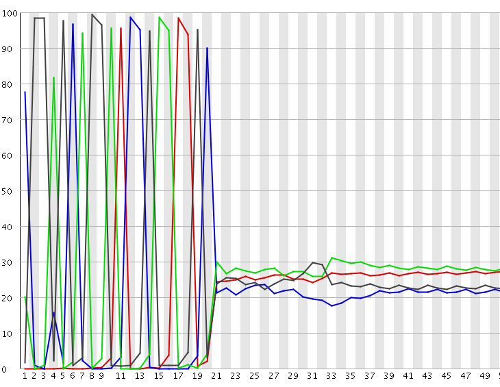
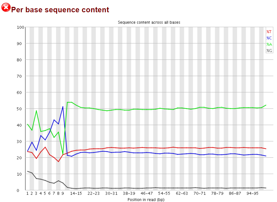
A per-base sequence composition plot from such a biased composition library is shown below. As you can see all reads in this library start with the same initial sequence, but then after 20 bases the sequences diverge.
In this type of library the symptoms observed will be any or all of:
- Poor overall sequence qualities
- Low cluster numbers, with a high number of clusters being rejected during the run
- A high incidence of ‘N’ calls in the output
- Higher than expected positional bias within the flowcell
Depending on the severity of the problem you may even get an almost complete failure of the run, although more normally you will get reduced yield with poorer quality calls.
Diagnosis
In order to understand the reason for these failures it is necessary to explain some of the steps in the illumina data analysis pipeline which relate to this problem. There are a few steps in the data collection which can be affected by these types of libraries:
1) Focussing
Illumina sequencing is an imaging based data collection. You have a glass flowcell onto which clusters of DNA molecules are attached, and after the addition of tagged nulceotides there is an imaging step where a computer controlled microscope images the surfaces of the flowcells. Right at the start of the run one of the critical steps in the data collection is to set the focussing for this flowcell. This focussing has to be done before the first data collection, so at the point of focussing only the first base in each cluster will be visible. The illumina system uses a number of different flurophore molecules and lasers to measure the different bases, but for focussing it just picks one of these channels to use, the idea being it doesn’t need to see every cluster, it just needs enough information to see the correct focal plane. If however you have little or no data in the channel being used to set the focussing then there is effectively nothing for the instrument to focus on, and it’s possible that the initial focussing will be so far out that it will never recover, generating out of focus clusters for the rest of the run with very bad knock on effects for data quality. The instrument does have the ability to adjust focus during the run, but this refocussing is limited to small changes, so if the initial focus is too far out it may not recover completely.
2) Cluster detection
On most illumina systems DNA clusters are randomly positioned over the surface of the flowcell (this is changing in more recent systems with the introduction of semi-ordered arrays of clusters) – so one of the other initial steps in processing is to identify where each individual cluster is on the flowcell so that it can be tracked through the run to produce an individual output sequence. When putting clusters on the flowcell there are two competing factors which need to be taken into account – ideally you’d like each cluster to be completely isolated from each other cluster so that as soon as you see a signal in the imaging you can assume that it comes from a single DNA sequence. However you also want to put as many clusters on the flowcell as possible to maximise the amount of data you get from a run. In practice therefore flowcells are loaded to a point where a significant proportion of the clusters will in contact with one or more other clusters such that a simple identification of the position of signals in the first sequencing cycle is not enough to identify the position of every individual cluster.
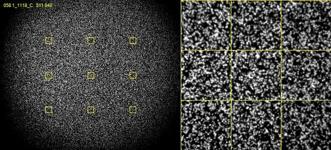
The way this problem is resolved is that cluster calling is not done solely on the data from the first sequencing cycle – instead data is collected from the first few cycles and each identified spot is analysed. If in any cycle a spot shows a pattern where, for example, the left side of the spot is mostly G signal, but the right side of the spot is mostly C signal then the system can assume that this is actually two spots which are touching and can treat the two halves as separate spots for future analysis.
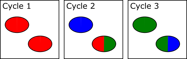
In the example below, both spots shown are actually two adjacent and touching clusters. The one at the bottom right can be distinguished as two clusters since the sequence within the two sub-areas changes within the set of cycles used for cluster detection, whilst the one at the top left has the same sequence through early cycles and will be analysed incorrectly as if they were a single cluster.
The problem with this approach is that there is a limit to how far into the run the system can detect these merged spots. After a spot is identified as being merged the system must go back to the raw image data for the two halves of that spot from the start of the run to call signal for the two regions separately. This means that until spot detection is complete all of the raw image data for the run must be kept, and this data is BIG! Practically therefore the spot detection can only run for a few cycles. For biased libraries the effect of this is that unless the library sequence for two overlapping spots diverges within the set of cycles used for cluster detection it will be considered as a single cluster for the remainder of the run. When the sequence eventually diverges it will appear as a mixed signal and the cluster will likely be discarded due to this.
3) Channel calibration
The final aspect to this type of failure is the calibration of the specific parameters used to base call each run. For optimal base calling the software needs to work out the relative strengths observed in the different measured channels in each run. This accounts for variations in the laser or detector efficiencies or in the properties of the fluors used in the libraries. Setting these calibtration values must, by design, make some assumptions about the nature of the nature of the data it expects to see, so when a library is hugely biased (possibly to the point where some channels are completely blank) it is perhaps not surprising if the paramters for the run are not set optimally, and base call quality is therefore reduced.
Mitigation
To some extent this problem has been greatly mitigated by improvements in the base calling software by illumina. Improvements in the focussing and calibration now mean that libraries rarely completely fail (which used to be a common occurrence on the GA sequencers), but loss of sequences, inclusion of N’s in the calls, and lower than normal phred scores are still common. Informatics improvements can only takcle some of these issues, ultimately some of them require changes in the libraries or sequencing reactions to fix.
Some common fixes to this problem are:
- You can spike diverse sequence into the library. Most commonly this will be the PhiX control library which Illumina themselves provide. Even a low (~5%) amount of this will give enough signal to fix the focussing and will improve the calibration. Higher amounts will begin to alleviate the cluster detection issue as you’re more likely to see overlaps between a fixed sequence and PhiX, but this obviously comes at the cost of wasting sequencing capacity on generating phix sequence.
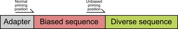
- You can restructure your library to not have a fixed sequence at the front. You can improve some aspects of the sequencing by adding a random barcode to the front of the insert, but fixed bases later in the library will still be a problem. If the random sequence can be made to be variable length then this will provide diversity for the rest of the library, and as long as you can identify the start of your insert this can provide a more complete solution.
- If your library has a completely fixed sequence at the start which later turns into diverse sequence then the easiest and most effective fix is to change the primer used for the sequencing to one which primes immediately upstream of the diverse region. This has a couple of advantages, it stops you wasting sequencing capacity sequencing the common sequence, and it means the library starts at a diverse position so the calibration and cluster detection will be good.
Lessons Learnt
Sometimes a good understanding of the methodology of your sequencing platform can help to understand sequencing failures and point to possible solutions.
References
Krueger F, Andrews SR, Osborne CS Large Scale Loss of Data in Low-Diversity Illumina Sequencing Libraries Can Be Recovered by Deferred Cluster Calling PLoS One. 6(1): e16607.
Mispriming in PBAT libraries causes methylation bias and poor mapping efficiencies
Introduction
In 2012, Miura and colleagues described a new method of preparing libraries for bisulfite sequencing termed Post-Bisulfite Adapter Tagging (PBAT). In this technique DNA is sheared by the bisulfite reaction itself, and the fragments that are later sequenced are regenerated by two rounds of random priming with random tetrameric (4N) oligos and strand extension. The undisputed advantage of this method is that a lot less starting material is needed which makes it amenable for rare cell types or even single-cell analyses. Several optimised PBAT-type protocols have since been published or are even available as commercial kits, e.g. the EpiGnome (epicentre) or Pico Methyl-Seq (Zymo) kits.
We and others have noticed early on however that most of these methods introduce a hefty bias in sequence composition at the 5′ end of reads, which corresponds in length exactly to the length of the oligo used for random priming (4N in the original paper, but methods often also use 6N, 9N or 12N). All examples shown in this article used a 9N oligo for the initial pulldown reaction.
The Symptoms
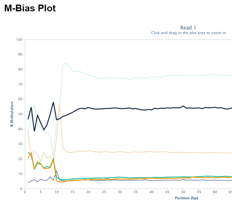
The biased sequence composition is also carried through to the aligned sequences (not shown here), and sure enough the methylation levels at the first couple of positions is also severely distorted, especially in non-CG context, as can be seen from the Bismark M-bias plot (please also see the M-bias plot in this post):
We never really got to root cause of the problem but were convinced that this has to be a technical artefact rather than a biological effect. We suggested to simply remove the first bases either by 5′ trimming the raw sequences, or by ignoring the first N bases during the methylation extraction.
Diagnosis
5′ trimming the 4N, 6N or 9N portion of single-end (SE) reads works like a charm for both mapping and M-bias plots, the data looks reasonably clean afterwards and one can achieve mapping rates of 60-70% for 100bp reads and mapping to the mouse genome (which is fairly good).
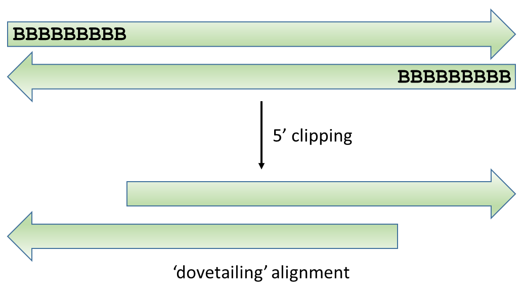
It gets a bit more tricky for paired-end (PE) reads however, because simply removing the biased positions (marked as B below) for both reads of paired-end alignments may result in ‘dovetailing’ reads, where one or both reads seem to extend past the start of the mate read. Bowtie2 alignments in Bismark are carried out invariably using the option --no-discordant so that really odd combinations of read pairs (such as oriented away from each other, only one read aligns, reads align to different chromosomes etc.) are not reported as valid paired-end alignments. Dovetailing alignments are also considered discordant and thus do not get reported.
This obviously only applies when the sequenced fragment is shorter than the sequencing read length, but as shown for the 2×10² bp (9N PBAT) example above there are quite a few alignments shorter than 100bp:
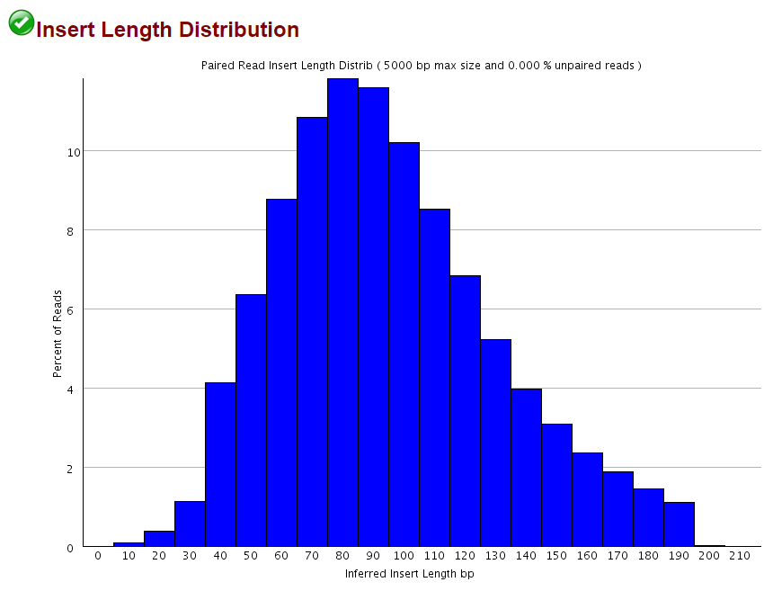
Since we knew that dovetailing reads were a problem we tended to run PE alignments without 5′ clipping the biased positions (just doing the usual adapter and poor quality removal using Trim Galore) and instead ran the methylation extractions with the options --ignore 9 --ignore_r2 9 to disregard the methylation calls from the first couple of positions. This effectively removes the horrible bias at the start but people were complaining about poor mapping efficiencies…
To find out whether we should align the data including the first positions (the argument being that they were genuine captured genomic sequences) or remove them before trimming we ran alignments with 5′ unclipped data and then looked at the rate of SNPs within the first couple of positions of the aligned data:
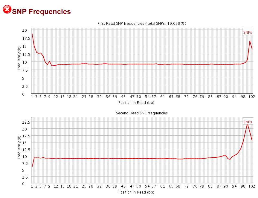
It was quite intriguing to see that the level of SNPs found in the first 9bp of Read 1 and last 9bp of Read 2 (corresponding to the start of R2) were drastically elevated. It has to be mentioned that the overall frequency of SNPs appears fairly high due to the presence of C->T conversions that are mere methylation changes rather than true SNP calls.
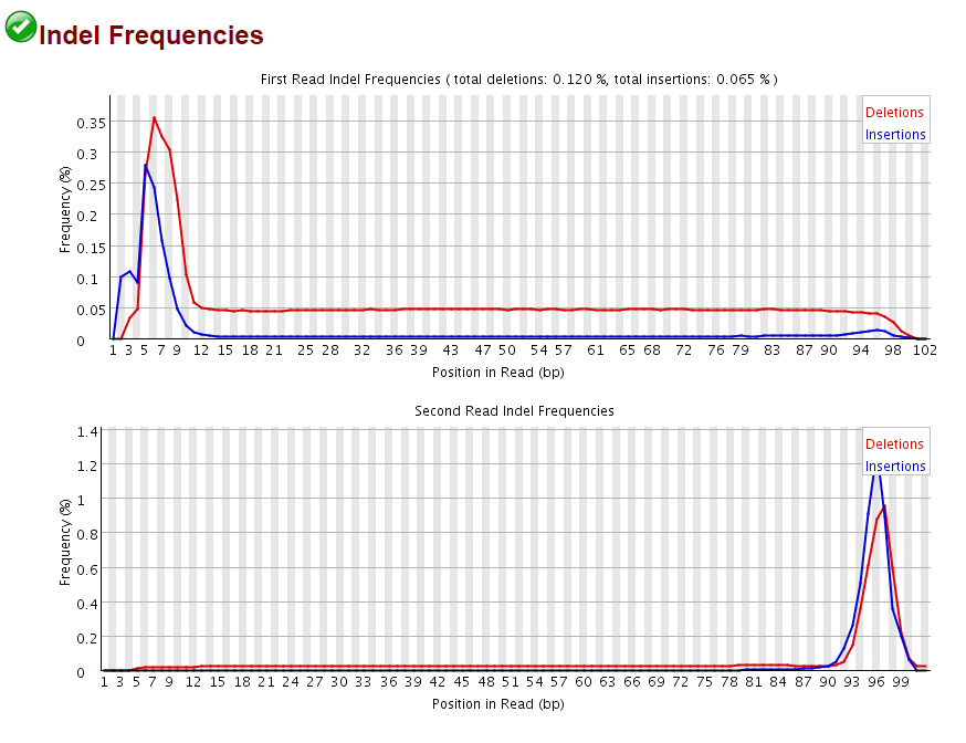
In addition the reads also sported a sharply increased frequency of insertions or deletions at the start of Read 1 and Read 2, again corresponding almost perfectly to the 9N random primed portion of the reads:
This demonstrated convincingly that there are weird things going on during the “random priming” step of the PBAT protocol, resulting in a drastically increased rate of SNPs and InDels. Since both SNPs and InDels make it more difficult to map a read we reasoned that this could be at least in part responsible for the poor mapping efficiencies observed for 5′ unclipped PE PBAT libaries. When the alignments were run again relaxing the mapping parameters (allowing three times as many mismatches and/or indels than in the default setting) the mapping efficiency did indeed increase dramatically from 39 to 58% (not shown). This demonstrated nicely that this library was largely comprised of valid paired-end alignments, but since we expect that a much increased rate of mismatches and indels at the start will also result in incorrect methylation calls we do not recommend relaxing the mapping parameters to remedy the low mapping efficiency of PE PBAT alignments.
Mitigation
To get around this issue we implemented a new option --dovetail into Bismark so that dovetailing alignments are now considered concordant. This allows us to run Trim Galore on the data specifying the length of the random pulldown oligos (here 9 bp) as parameter for 5′ clipping, e.g. with a command like this:
trim_galore --clip_R1 9 --clip_R2 9 --paired sample_R1.fastq.gz sample_R2.fastq.gz
This of course auto-detects and removes read through adapter contamination and poor basecall qualities as well. Running test alignments with Bismark/Bowtie2 and default parameters with either i) unclippped regular alignments, ii) 9 bp 5′ clipped regular alignments or iii) 9 bp 5′ clipped alignments with --dovetail gave the following results:
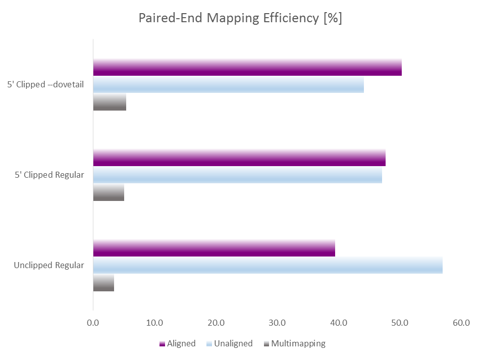
Merely clipping 9bp of the 5′ end already increased the mapping efficiency from 39 to 47% which is in line with removing lots of inhibitory indel and SNP errors within the 9N random priming part. Allowing dovetailing alignments with --dovetail increased the mapping efficiency further to > 50% while at the same time lowering the rate of (probably contaminating) non-CG methylation levels (not shown).
As a result of this the option --dovetail will now be turned by default whenever --pbat is selected in Bismark (version 0.15.1 and higher, available from the Bismark GitHub page).
Prevention
As long as there are no major changes in the PBAT protocol the problems described in this article are unlikely to go away. We do recommend 5′ trimming of the random priming portion of reads in addition to removing standard read-through adapters and poor qualities before aligning the data. Specifying --pbat in Bismark will automatically set --dovetail as well so the default mode should do just right thing from now on.
A word about hybrid reads in PBAT libraries
While the measures described above should be pretty effective in combating errors introduced by the PBAT protocol it should be noted that we have seen a tendency of hybrid reads in PBAT libraries. Hybrid reads in this context are reads that would be considered discordant, i.e. where R1 and R2 align to completely different places in the genome. These reads will not be reported by Bismark as valid alignments, but we have seen paired-end libraries with in excess of 30% of all fragments aligning as to different places in the genome similar to a bisulfite Hi-C experiment (should there be one…). It is debatable whether a read pair starting at say chromosome 3 and continuing into chromosome 17 contains credible methylation information, but clearly a fairly large portion of hybrid reads seems to contribute to the generally low-ish mapping efficiency observed for some PE PBAT libraries.
As a solution to this problem we would probably recommend to run 5′ clipping and trimming first, and run PE alignments with --unmapped specified in Bismark. The resulting unmapped Read 1 and Read 2 files may then be aligned in single-end mode afterwards to salvage as much data from alignable hybrid reads in the experiment as possible (--pbat for R1 and default settings for R2).
Lessons Learnt
I think we have now finally got to the bottom what causes the weird biases in PBAT-type libraries. It is important that the community understands that the problems associated with the biased positions and takes appropriate measures (a typical lane of HiSeq may potentially result in several (hundred) million incorrect methylation calls otherwise…).
Side Note – Bias on the 3′ end
One could argue that the bias described above exists on both sides of fragments because the 3′ end is going to be filled in by a copy mechanism from the other, biased, strand. While this is probably true it seems that elimination of the bias on the 5′ end is much more relevant because of the following reasons:
- the 5′ bias affects potentially all reads
- the 3′ bias is only sequenced if the fragment length is shorter than the read length. Depending on the library preparation this may only be a small subset of the total library
- we don’t see a distinct increase of SNPs, indels or M-bias changes towards the end of reads, even though this could be masked by different the read ending at different positions. (The peak in SNPs for Read 1 in the example above probably stems from a rather low amount of sequences with that length, and might in fact be caused by adapter trimming)
- the 3′ end is subject to adapter/quality trimming, and thus for short enough fragments the bias may have been removed already by the quality trimming step
- the 3′ bias of Read 2 would not be counted anyway because as soon as reads start overlapping the methylation calls of R2 are ignored during the methylation extraction
So in summary, at the current time we believe that only ever half (R1) of a subset (short) of a subset (not quality trimmed) of total reads might affected by a bias on the 3′ end. In other words, it might be a source of error one can live with.
References
Original paper describing the PBAT method. Miura et al., 2012.
Datasets
No dataset specifically, but any PBAT library we have seen so far exhibited the same problems. Just find one on GEO.
Software
QC plots were generated with FastQC or BamQC.
Adapter/quality trimming and 5′ clipping was performed with Trim Galore.
Bisulfite reads were aligned and plots generated using Bismark (on GitHub).
Data can be corrupted upon extraction from SRA files
Introduction
Its is a common practice to re-use data deposited in one of the large public repositories. In some cases only highly processed quantitated data will be used, but often it is better to go back to lower level formats such as fastq files to run your analysis. In these cases we rely on the repository providing accurate data from which we can work but there are a number of ways in which this can fail.
One of the most problematic steps in the re-use of public data is extracting the fastq files from the database. The NCBI short read archive uses their own format, the SRA file, to store primary data. The SRA file is a composite file, much like a zip or tar file, which can contain multiple data sources within it, and NCBI provide a suite of tools, the sratools package to manipulate these files.
One of the most common operations on sra files is to extract the individual fastq files from the archive. For this process you use the fastq-dump program. If your data is paired end then you need to add the –split-files option to the program so that it writes out each read into a separate file. Omitting this will simply concatenate read 1 and read 2 in a single file, indicating that the internal representation of the read data in the file is simply a concatenation of the different reads.
Although this process works fine most of the time we have seen several cases where incorrect metadata in the repository leads to incorrect extraction of data from the file. Unfortunately this pretty much always still allows the extraction to complete without generating and errors or warnings so the issue may only be spotted later in an analysis pipeline.
The Symptoms
Although the failure here will probably be spotted in a larger pipeline by errors at the trimming / mapping stage it is first evident in the extracted fastq files. The obvious symptom is that the reads extracted will not have the expected length, and may contain odd characters (often a # symbol) in place of base calls.
For example if we have a look at sample SRR2133905. I can pull down the sra file from NCBI, and run fastq-dump successfully on it, but if I look at the files created then I see an odd split of data:
$ head -4 SRR2133898_Worker_3_Transcriptome_1.fastq SRR2133898_Worker_3_Transcriptome_2.fastq
==> SRR2133898_Worker_3_Transcriptome_1.fastq <==
@SRR2133898_Worker_3_Transcriptome.1 HWI-ST412:281:D1D1BACXX:2:1101:1515:2212 length=98
TCGGATTCGTTCGATCCTTTTTTAAAGCTGACGATTTTTCTTTTTCTTTTCTTTTTCATCTAACGTGTTATTTTTGTTCTCTTTCTCTCTCTATCTCT
+SRR2133898_Worker_3_Transcriptome.1 HWI-ST412:281:D1D1BACXX:2:1101:1515:2212 length=98
@<@DABDBFFHFH:CGCCHHCHHG?4?<3C3:)00BDEG*?DGGE88BGA)8)8@F@;;CCE####################################
==> SRR2133898_Worker_3_Transcriptome_2.fastq <==
@SRR2133898_Worker_3_Transcriptome.1 HWI-ST412:281:D1D1BACXX:2:1101:1515:2212 length=1
C
+SRR2133898_Worker_3_Transcriptome.1 HWI-ST412:281:D1D1BACXX:2:1101:1515:2212 length=1
#
You can see that read 1 has a length of 98bp and read 2 has a length of only 1bp, which doesn’t seem right. I can do the dump again, but without splitting files and get this:
$ head -4 SRR2133898_Worker_3_Transcriptome.fastq
@SRR2133898_Worker_3_Transcriptome.1 HWI-ST412:281:D1D1BACXX:2:1101:1515:2212 length=99
TCGGATTCGTTCGATCCTTTTTTAAAGCTGACGATTTTTCTTTTTCTTTTCTTTTTCATCTAACGTGTTATTTTTGTTCTCTTTCTCTCTCTATCTCTC
+SRR2133898_Worker_3_Transcriptome.1 HWI-ST412:281:D1D1BACXX:2:1101:1515:2212 length=99
@<@DABDBFFHFH:CGCCHHCHHG?4?<3C3:)00BDEG*?DGGE88BGA)8)8@F@;;CCE#####################################
..which suggests that the sra file only contains data for 99 bases.
Diagnosis
To try to understand this I can go digging into the submission files. We can first look at the NCBI experiment details which show the following:
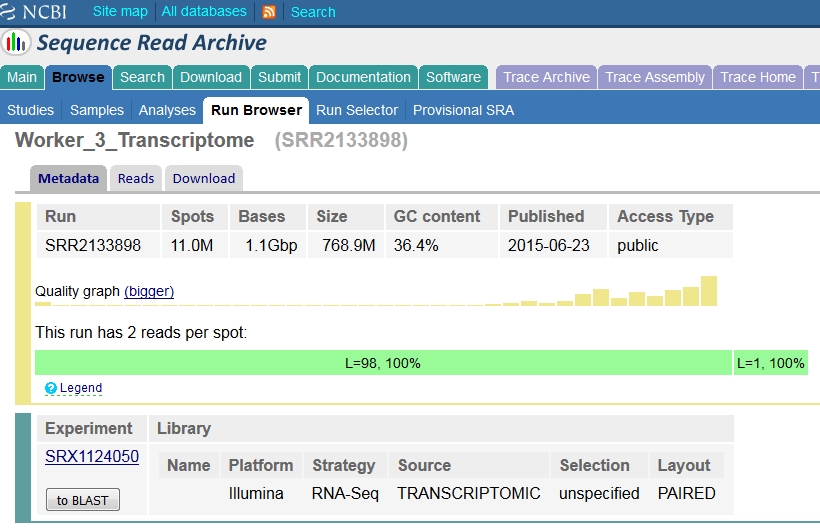
So the metadata here agrees with what we get from the extraction – a read of 98bp and a read of 1bp, but this doesn’t seem right. If we go to the metadata file at the ENA we see:
<SPOT_DESCRIPTOR>
     <SPOT_DECODE_SPEC>
          <SPOT_LENGTH>196</SPOT_LENGTH>
          <READ_SPEC>
               <READ_INDEX>0</READ_INDEX>
               <READ_CLASS>Application Read</READ_CLASS>
               <READ_TYPE>Forward</READ_TYPE>
               <BASE_COORD>1</BASE_COORD>
          </READ_SPEC>
          <READ_SPEC>
               <READ_INDEX>1</READ_INDEX>
               <READ_CLASS>Application Read</READ_CLASS>
               <READ_TYPE>Reverse</READ_TYPE>
               <BASE_COORD>99</BASE_COORD>
          </READ_SPEC>
     </SPOT_DECODE_SPEC>
</SPOT_DESCRIPTOR>
So this run is supposed to have (according to the metadata) 196bp of data, split into 2x98bp reads. We can start to see where the issue arises therefore. The fastq-dump file knows that read2 is supposed to start at position 99, so it splits its read string there, but because there are only 99bp instead of 198 we get a very truncated read 2.
There are two possible reasons for this problem therefore, either there is read data missing, or the metadata is wrong. Since this is an RNA-Seq run we can use the properties of the data to try to distinguish these two options.
A simple check is whether the same data comes down from a different repository. We can pull the fastq files from ENA. If we do this we again find a 98bp read and a 1bp read, so at least the problem is consistent.
One of the notable things about RNA-Seq data is that due to biased priming you get sequence composition bias at the start of each read. If the data we have contains both read 1 and read 2 we should therefore see this bias at the start of the data, but see it again in the middle. When we run fastqc on the unsplit data we see the following:
So there is no evidence for a second set of biased positions, suggesting that we’re simply missing data. Interestingly we don’t even see a bias in the last position which suggests that the 99th base may not be the first base of the second read either.
Going back to the original paper we find the material and methods say:
10986225 reads; of these:
  10986225 (100.00%) were unpaired; of these:
    1142174 (10.40%) aligned 0 times
    8766188 (79.79%) aligned exactly 1 time
    1077863 (9.81%) aligned >1 times
89.60% overall alignment rate
Mitigation
In this case we can proceed using just the read1 data. We can pursue the rest of the data with the sequence repositories and the original authors to try to get a more complete dataset.
Prevention
This type of error should really be prevented during the submission process to the public repositories. Some simple data validation would have shown that the available data could not possibly match the metadata and yet two repositories provide this invalid data for download.
Lessons Learnt
I guess the message here is don’t automatically trust data from public repositories, and always try to validate that data and metadata match. You should also not always rely on program which fail (such as fastq-dump here) actually throwing an error. The exit code for the extraction was 0 in all cases so it wasn’t caught by our normal monitoring.
Datasets
The accession used here is SRR2133898 and the data shown was from 3 Mar 2016. It’s possible that this entry will be corrected in future if the full dataset is submitted.
Barcode splitting doesn’t work as expected
Introduction
Most sequencing platforms have the ability to generate way more data from a single sample than would be required for many types of experiment. Rather than waste the extra sequencing capacity it is very common to mix samples together so that multiple samples can be run in a single sequencing lane. In order to be able to separate the data coming from the lane modified adapters are used which contain a sample specific DNA tag called a barcode. Depending on the platform these barcodes might appear at the start of the normal sequence read, or they might be separately sequenced in a separate sequencing read. In any case the idea is that by reading the barcode sequence from an individual read and matching it to the set of barcodes used in the lane you can split the data back into the individual libraries which were mixed together.
This early stage of processing is one of the most common places to have problems with data processing and there are some very common modes of failure which can potentially lose large amounts of valid information from a run.
The Symptoms
The most common and obvious symptom that there was a problem with barcoding is that one or more samples end up with very little data in them. In these cases unless you have an easy way to investigate the details of the barcode splitting it can be difficult to ascertain whether the failure is a real problem with the sample, or simple a processing error with the barcode splitting.
On some sequencing platforms the barcode splitting is done as part of the early stage data processing, so end users may not be able to see the details of what happened, but finding a way to get to the composition of the barcode reads and looking how these relate to the expected samples can be invaluable in determining what has gone wrong.
Diagnosis
The plot below shows the sort of information you need to be able to evaluate how well a barcode split has gone. This particular plot is generated by the Babraham Institute’s sequencing pipeline, but similar plots could be constructed from the raw barcode splitting metrics which should be available on most sequencing platforms.
This plot shows the set of barcode sequences which were most frequently observed in the dataset (anything over 1% of the data). The barcodes which were listed as being present in the sample are highlighted in red and anything in grey is unexpected. At the top of the plot you can see the proportion of the whole dataset which is shown in the plot – this can be useful for determining if there is a large amount of reads with very variable sequences.
Ideally what you’d like to see in these plots is only the expected barcodes, and all of them with the same frequency. In practice balancing samples in a lane is not an exact science so some variability between barcodes is to be expected.
In the plot above the unexpected barcode comes from a PhiX spike in control added to the lane, so this is fine and means that the sample should be OK to process. In many cases though the splitting does not work smoothly.
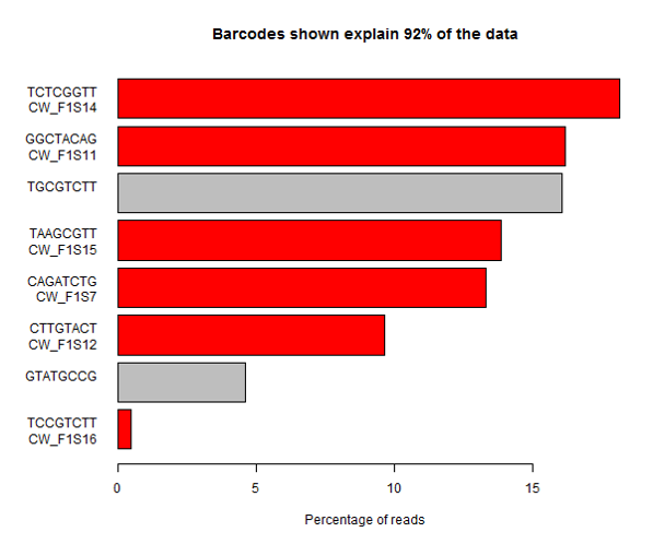
In this sample you can see that one of the expected barcodes is present at a very low level (not zero though), and there is an unexpected barcode taking up a large proportion of the lane. If you are not able to see the barcode splitting stats for this data then you might assume that one of the samples had failed, or that the sample mixing had been poorly calculated. It’s only by looking at the whole picture that you can see that in this case it’s more likely that the barcode has simply been mis-typed when creating the sample sheet and that the data was present in the lane, but has been incorrectly discarded.
A more extreme version of this problem is shown here. In this case all of the expected barcodes are very low, and there are a set of unexpected sequences observed. The problem here was that although the user added the correct sequences, they got them in the wrong orientation, so that the actual sequences produced were the reverse-complement of what they expected. This type of error is very easy to make if users have to actually enter the sequences of barcodes, rather than entering something more abstract such as a tag number.
In addition to these relatively simple cases there are more subtle things which can go wrong in barcode splitting which can be very difficult to track down. The image below shows the barcode splitting summaries from a number of datasets from the same group run over a number of months. Have a look at the results and see if you can spot a problem, and identify which sample or samples are affected.
The answer here is that all of the datasets have a problem, but because of the way the barcodes were used it only becomes apparent in the final dataset. What we see in the last dataset is the presence of an unexpected barcode (TTA). In this case this wasn’t a known spike-in, so there was no obvious explanation for where it had come from. It’s temping to ignore these types of minor contaminant and continue to work with the rest of the data, but it is worth tracking down these sources of contamination.
In this case the reason for this extra sequence is that the barcode stock for the CGA barcode had become contaminated with TTA, so whenever a CGA tagged sample was put into a run, around a third of the reads from that sample would actually have a TTA barcode. The reason this hadn’t shown up before was that all of the previous runs had used both TTA and CGA in the expected barcodes. Knowing about this contamination we can see that there is a general bias for TTA tagged samples to have more reads than average, and CGA to have fewer reads than average, but never enough of a discrepancy in an individual experiment to cause concern.
The effect of this type of problem is really quite bad though. It means that the data from all TTA tagged samples is mixed with whatever was tagged with CGA, and there is no way to separate them. In the actual case from which this example is drawn this meant either re-analysing data excluding the contaminated samples, or rerunning them with a barcode combination which would allow them to be correctly split. Needless to say, even though this type of confusion is potentially very serious, it is also very easy to miss.
Prevention
Ultimately barcode splitting problems are going to happen and there’s little you can do to completely prevent mistakes from happening. There are a number of steps which will help though.
- Ensure that you correctly monitor and report on your barcode splitting. This means that the data you extract from a lane must be put in the context of everything which was observed in that lane. In particular don’t ignore the reads which went into the discard pile – these normally contain the critical information you need to quickly diagnose problems with the splitting.
- When creating systems to handle samples and barcodes try to make correct entry of codes as simple as possible. Ideally give people a way to enter tag names / numbers rather than entering sequence. If they do have to enter barcode sequences then do sanity checks on the sequences entered: Are the sequence all the same length, are there any duplicates, are there any non-GATC characters etc.
- Whilst there are definitely good practices about which combinations of barcodes to use, try not to always stick to the same subset of barcodes, mix around the combination of codes used where possible, and be suspicious if certain codes produce consistent contaminants, or are consistently over-represented in the data.
Lessons Learnt
Barcode splitting seems like a trivial part of the data analysis pipeline, but it’s one of the most frequent causes of error. Adding QC and sanity checks to this step can normally identify problems very quickly and save a lot of wasted effort downstream.
Library end-repair reaction introduces methylation biases in paired-end (PE) Bisulfite-Seq applications
Introduction
Library construction of standard directional BS-Seq samples is a multi-step process typically consisting of several consecutive steps:
- Sonication
- End-repair
- A-tailing
- Adapter ligation
- Bisulfite conversion
The end-repair step typically uses a mix of nucleotides to fill in fragments with a 5′ overhang which are frequently generated by sonication, leaving blunt ended fragments ready for the A-tailing procedure. This would not be apparent in other applications such as ChIP-Seq or RNA-Seq because the genomic sequence is simply regenerated in these fragments. The situation changes in BS-Seq applications though because it does not really interrogate the sequence itself but the methylation state of cytosine residues. The nucleotide-mix used in the lab typically uses a standard mix of the four nucleotides C, A, T and G for the fill-in reaction, whereby C is typically unmethylated for cost reason.
The Symptoms
This schematic drawing shows that cytosines located towards the 3′ end of reads may be filled in with unmethylated cytosines during the end-repair step. Since the fragments undergo bisulfite treatment after the adapters have been ligated on, these cytosines (marked in red) will be converted to T. Since Read 2 starts right from this end carrying the artificial bases they will be (incorrectly) read as unmethylated cytosines. If the sequenced fragments happen to be very short you might also see a read these filled-in positions at the 3′ end of Read 1, but this will be arguably quite rare, whereas the Read 2 bias definitely affects every single molecule with filled in cytosines.

It is actually pretty much impossible to spot the symptoms of this bias unless you really look for them as a post-alignment QC step (see below).
Diagnosis
The trouble with this kind of bias is that it only becomes apparent when you really look for it. To spot the bias one has to look at the average methylation levels across the entire length of the reads and plot out a methylation bias (or M-bias) graph:
Read 1 looks fairly normal with a little bit of a ‘wobble’ at the 5-end but generally fairly even methylation levels across the entire read.
Read 2 however tells an entirely different story:
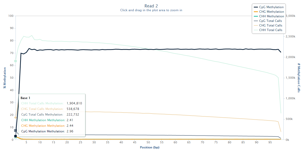
The methylation state of the first couple of bases or Read 2 drops from the average ~70% down to ~3%, and this steep drop can certainly be explained by the filled-in unmethylated cytosines. Since there is no reason to believe that there would be a biological role for lower methylation at the start of reads we have to assume that this low-methylation is artefactual, and thus leaving this untreated will introduce, in this case several hundred thousand, incorrect methylation calls (and thus noise) into the dataset.
Mitigation
Fortunately it is relatively easy to fix this problem by simply disregarding the biased positions when running the methylation extractor. Since this problem only affects Read 2 of paired-end libraries a typical command like this should fix the problem:
bismark_methylation_extractor --ignore_r2 2 --gzip sample1_bismark_bt2_pe.bam
The same M-bias plot for Read 2 should then look like this:
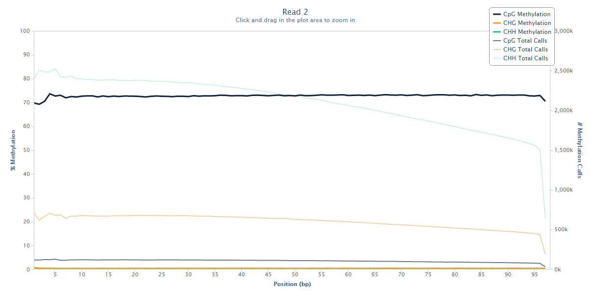
Prevention
Since this is a common phenomenon with any standard directional library the option –ignore_r2 2 of the methylation extractor should be added to the default data processing pipeline for paired-end applications.
Lessons Learnt
Read 2 of paired-end BS-Seq libraries suffers from artificial hypomethylation at the start of Read 2 of paired-end reads. This will add spurious hypomethylated calls and should be removed from the dataset before proceeding to downstream analysis.
References
The M-bias plot was first described in this paper: Hansen et al., Genome Biology, 2012, 13:R83
Datasets
Any paired-end directional BS-Seq dataset will show this problem.
Software
To get to the stage where you can see the M-bias plot data was adapter and quality trimmed with Trim Galore and aligned to the mouse genome using Bismark. Methylation information was extracted using the bismark_methylation_extractor and reports shown in this article were generated using bismark2report.
Deduplicating ambiguously mapped data makes it look like repeats are enriched
Introduction
Repetitive regions are one of the most tricky areas of the genome to work with and yet are also potentially very biologically interesting. When analysing any type of enrichment experiment people are often interested to look at the repeat sequences to see if anything interesting comes up. Unfortunately these regions are prone to producing technical artefacts, and in some cases these can be very convincing.
The effect described here occurs in any library where there is some degree of technical duplication. Additionally the reads must not have been filtered to retain only uniquely mapped reads (ie keeping one randomly selected position from the set of possible mapped positions), and the data must have been deduplicated.
Under these circumstances repetitive elements in the genome will appear to be enriched. The amount of enrichment can be quite high (it’s proportional to the amount of technical duplication, so bad libraries appear more enriched), and the effect is very well localised to the repeat elements. It is very easy to become convinced that you’re seeing a true biological enrichment.
The image below shows a SeqMonk aligned probes plot for the full length instances of LINE1 repeats. Each line is one repeat instance, and the depth of colour represents the number of reads mapping to that part of the sequence. You can see that in the green ChIP plot there is a strong enrichment over the repeat which starts abruptly at the start of the repeat. In the corresponding input sample on the right there is a slight enrichment, but nowhere near the amount seen in the ChIP.
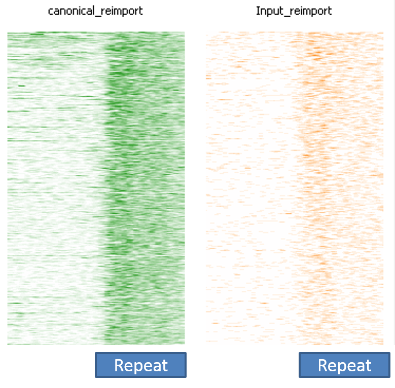
This impression of biological validity is further enhanced by the fact that the enrichment only really happens over full-length LINE1 instances. Partial copies do not show anywhere near as much enrichment.
Unfortunately this effect is completely technical and there is no true enrichment. The underlying cause is how ambiguously mapped reads are handled.
If we consider a simple case such as the one below where we have one non-redundant region (in green) and two copies of a repeat (in blue), and in each of them we have a single region sequenced, but this has been PCR duplicated so we get two reads over each position.

The problem is that our read mapper can’t tell the difference between repeat 1 and repeat 2 since they’re the same sequence. When presented with multiple options for where to position reads the default action for most read mappers is that they randomly select one of the valid positions and report that (whilst lowering the mapping quality value reported). This means that the mapping we actually get might well look like this:
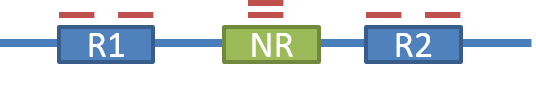
The non-redundant reads will both have been positioned correctly, but the repetitive reads will have been split between the two repeat instances.
If we now deduplicate the data then we get this:
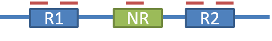
Because the non-redundant reads were positioned correctly they were also correctly deduplicated to leave only a single read, but because the repetitive reads were spread over the different repeat instances the PCR duplicates didn’t end up at the same genomic position, and both copies survived deduplication. Overall then we should have had one read in the NR region and two in the repeat regions, but we had 4 in the repeats instead, leading to the impression that the repeats are enriched for reads.
In real data you will also see that complete copies of larger repeats will exacerbate this effect, with partial repeats appearing less enriched. This has nothing to do with the biology of the repeats and simply reflects the fact that complete, active repeat copies tend to be more similar to each other than partial copies which can degrade, and therefore become more distinct from each other and more likely to be uniquely mappable.
Mitigation
In these cases the effect would not be present if the data had not been deduplicated, or if the reads had been pre-filtered for unique mapping. Filtering for uniquely mapped reads will actually deplete the repeat regions of reads, but in a way which should be the same for different samples regardless of their technical duplication level.
Prevention
This effect can be prevented fairly easily once you know that the effect exists. One of the problems we’ve seen is that people who were aware of the effect could still suffer from it if they were unwittingly performing a deduplication. For example, many peak callers (for example MACS) include a deduplication step in their internal analysis pipeline, so even if you don’t explicitly deduplicate your data, you can still end up with biased sets of peaks.
Lessons Learnt
Repeats are icky. Always be super-cautious when making conclusions about their behaviour.
Software
The data plot shown in this article was created with SeqMonk.
Read-through adapters can appear at the ends of sequencing reads
Introduction
A sequencing library consists of a set of DNA fragments for which sequence is to be obtained. Many sequencing platforms cannot sequence the DNA directly, but require the addition of platform specific adapter sequences to the ends to provide anchorage and priming points for the sequencing chemistry reactions. The sequencing reaction is designed so that the primer will anneal immediately upstream of the insert to be sequenced, so the first sequence to be generated is the desired insert sequence, and not the adapter.
In some cases the length of the inserts in the library might be quite short – short enough that in some cases they are shorter than the read length of the sequencing run. Where the read length exceeds the length of the insert then the read will run off the end of the desired sequence and into the adapter on the other end. This will lead to the addition of non-native sequence on the end of some reads in the library. These will appear at various positions within the length of the reads, but will always consist of the same sequence. In the diagram below the red regions of the reads would be read-through adapter.
The Symptoms
The addition of artificial adapter sequence on the end of reads in a library will normally cause those reads to fall out of any downstream analysis fairly quickly. The bases in the adapter sequence will generally have high phred scores as there is no reason for the sequence to be of poor quality. They will introduce large numbers of mismatches into any genomic alignments causing affected reads not to map to reference genomes. Assembly with these reads will likewise fail since proper extension will also fail at the point where adapter sequence is reached.
Diagnosis
Since the sequence of the adapters used for a given library is known ahead of time, and that sequence is normally not present then it is possible to explicitly screen for that sequence within the library to identify which reads contain adapter and at what distance into the read. Since the number of different adapters used by the major platforms is relatively small it is even possible to screen for all of the normal adapter sequences as a matter of course. This will both check for the presence of adapters in the library and also confirm that it is the expected adapter which has been found.
Mitigation
Adapter trimming is the standard approach to removing adapter sequence from sequencing libraries. In this process a search is performed for the adapter sequence within each read, and the read is truncated to the point where the adapter is found to start. This kind of trimming is easy when there is a substantial amount of adapter present since there is only a low likelihood that this could be native sequence. It becomes more difficult where the added length of adapter is relatively short (only a few bases) since small numbers of bases consistent with being adapter could easily be present on the end of a native sequence. There are a few options in these cases:
- Aggressive adapter trimming – you can choose to remove even the shortest amounts of adapter from the end of all reads. This should provide fairly complete removal of adapter sequence, but will also trim back native sequence where the end of the read coincidentally looks like short amounts of adapter. This kind of aggressive trimming may be preferred where small amounts of adapter could have a deleterious effect on downstream analysis, such as for SNP detection or for detection of methylation in bisulphite sequencing. This kind of trimming will also introduce a sequence bias into the end of libraries which can trigger warnings in other QC. For example if the first base of an adapter is a T then no full length sequence will be allowed to end with a T since this could represent a 1bp adapter read-through so you should see a complete depletion of T in the last base of the full read length.
- Limited adapter trimming – you can set a threshold for the amount of adapter which must be present before being trimmed. Requiring the presence of several bases of adapter which continue to the end of the read will reduce the amount of over-trimming you perform, but will mean that some short adapter regions will remain in the library. If the nature of the library is such that the mismatches from these short adapter stretches could be significant then you might want to use a more aggressive trimming strategy.
- If you have performed paired end sequencing then you can use the information from the other end of the pair to decide on the exact position of the adapter. If you sequence long enough to read right through the insert in read 1, then you would read past the point where read 2 would start from (but on the opposite strand). In these cases you can actually align reads 1 and 2 and this will allow you to determine the exact extent of the true insert, which will run from the start of read 1 to the start of read 2.
Prevention
The only way to prevent adapter read through would be to either make the inserts longer, or to reduce the length of the sequencing reads performed. On many platforms there is a practical limit to how long insert sequences can be, and in many cases short inserts reflect underlying biology, so the need for adapter removal may well be around for the foreseeable future.
Software
The presence of read through adapters can be screened for with FastQC. There are many trimming programs available which all operate in roughly similar ways. We use (and wrote) trim galore which is designed to automatically detect the correct adapter to trim by looking into the data. It itself is a wrapper around the cutadapt program which does the actual trimming.
The detection and removal of unknown adapters in paired end data can be performed with skewer.
Libraries can contain technical duplication
Introduction
One of the central assumptions of the analysis of sequencing data sets is that each read counts as an independent observation, and that it comes from a separate biological molecule in the original sample. Statistics based on counts will only produce valid p-values if this assumption holds true, so anything which causes this assumption to be violated is a problem in the analysis. Because of the small amounts of material being used, most library preparation protocols still contain at least one PCR step to amplify the library, and this introduces the possibility that multiple sequences in the final library can arise from the same original fragment. Where this type of technical duplication is extensive then the results of analysis can be severely compromised so it’s important that such duplication is identified and, if possible, removed.
The Symptoms
As with many other biases, technical duplication in samples will not cause analysis pipelines to fail. The only effect will be that the results produced at the end of the pipeline are of poor quality, so it can be an easy effect to miss unless you specifically check for it.
If you look at the raw mapped reads for a relatively low density sample, significant amounts of technical duplication are normally easy to spot. Instead of seeing randomly positioned reads what you would observe would be a set of towers of reads where each read would be repeated a number of times, even though the sample as a whole was far from saturating coverage of the region it’s in.
In the example below the samples at the top show technical duplication, with each read being present 2 or 3 times. The samples at the bottom are not duplicated and most reads are in a unique position.
The big problem with identifying and removing technical duplication is that it’s not possible to always assume that two reads falling at the same point are the result of technical duplication. When the overall read density in a region gets too high then you will start to see co-incidental duplication from different biological molecules. For regions with very high read density therefore a simplistic measurement of duplication will confuse high biological read depth with technical duplication.
Diagnosis
Other than a manual examination of the raw data (which is always a good idea) there are some automated ways to look at the duplication levels of samples. At the sequence level programs like FastQC can look at the amount of observed duplication to produce plots like this:
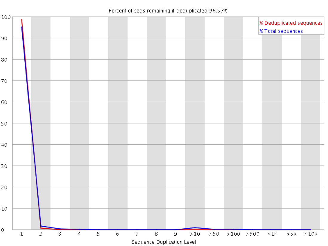
In this plot you can look at the proportion of reads in the library which arise from sequences which occur different numbers of times. In a truly diverse library like this nearly all of the sequences in the library occur only once. The headline figure at the tops tells us that only around 3% of reads would be lost if the library were to be deduplicated.
These sorts of plots can be misleading in a couple of ways through. If you have sequenced your library to only a low level then even if the library is moderately duplicated this will not show up since analysis of duplication requires sufficient read depth to observe it. Likewise if you sequence your sample to very high depth then you will end up with everything appearing duplicated to a similar level, but this could all be biological and not technical. The extreme example of this below is the duplication plot from running a whole lane of sequencing on the small bacteriophage PhiX. Every possible position will be observed thousands of times, but this is not necessarily an indication of technical duplication.
The observation of duplication is further complicated in library types where you do not expect that all regions being measured should be present at an equal amount in the sample. Any sample containing enrichment will have a different expectation of biological duplication depending on the region a sequence comes from. In an RNA-Seq sample for example the expected duplication level will change depending on whether a read comes from an exon, intron or intergenic region, and based on the expression level of the gene it is in. Some regions will be enormously dense with reads, whilst others will be almost empty. This means that at a sequence level the interpretation of duplication plots is very difficult, and a proper diagnosis of duplication will need a more nuanced approach.
The key to evaluating technical duplication in samples which might be biologically saturated is to look at the relationship between duplication and read density. Biological duplication should be a function of the overall density of reads in a region – as the density increases so does the duplication level as random clashes become more frequent. Technical duplication on the other hand will be present at a similar level regardless of read density since it happens independently to each read. If we therefore plot duplication against read density, even in samples with wildly variable densities, we should be able to diagnose technical duplication.
In a sample with variable density, and no technical duplication you might see a plot like this:
Here you can see that there is duplication present – there are regions with >80% duplication, but you can also see that there are regions with low duplication, and that there is a direct relationship between the overall read density and the amount of duplication seen.
In contrast if you look at a similar sample which has suffered from technical duplication the plot looks very different:
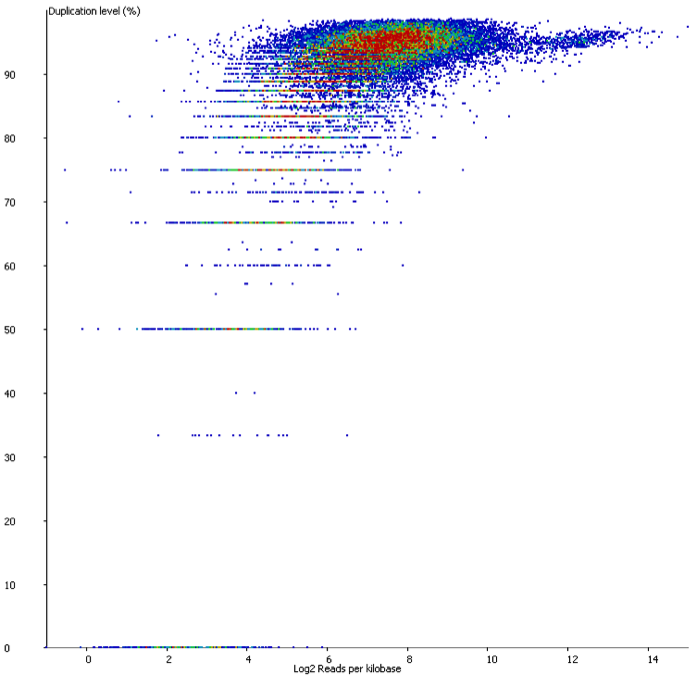
In this case the relationship between duplication and read density has disappeared. Even relatively low density reads have duplication levels of 50% or more and this should be a warning that technical duplication is present.
Mitigation
When thinking about the mitigation for duplication it’s worth thinking about why duplication is a problem. There are two main concerns with technical duplication:
- Technical duplication will artificially inflate the number of observations you appear to have. Any statistical analysis based on counts will have unwarranted amounts of confidence in measures coming from duplicated data due to the repeated observation of the same fragments. This will result in artificially low p-values and over-prediction of hits which are then likely to contain an inflated number of false positives.
- If the duplication you get does not apply equally to each fragment, but prefers some over others, then you might introduce a systematic bias into the data.
The mostly commonly used mitigation for duplication is de-duplication. In this process any place where multiple reads map to the same position in the reference genome will have all but one of these reads removed to completely remove the duplication. The problem with this approach is that it isn’t able to distinguish biological from technical duplication and both are removed. In samples where an even read coverage is expected and the depth of sequencing hasn’t come close to saturating this then this is a reasonable approach, but in samples with variable read densities this will have the effect of capping the maximum read density able to be obtained, and limiting the dynamic range able to be obtained. If multiple samples with different amounts of technical duplication are deduplicated in this way then you will actually introduce differences where the don’t exist.
The plot below shows the effect on quantitation of deduplicating a sample which had no technical duplication. You can see that the loss of value in the quantitation is not even, but is proportional to the read density.
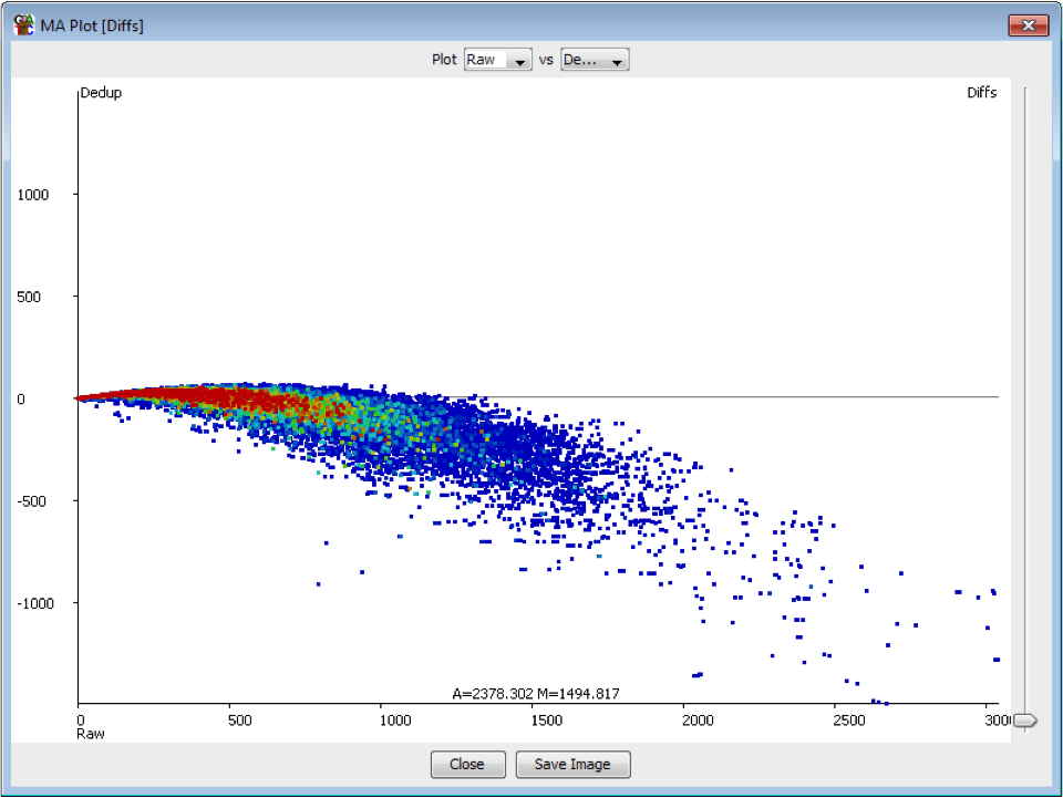
In general therefore deduplication is not appropriate if you have samples with variable coverage where you want to keep a fair quantitation between high and low density regions.
If your concern is with the inflated increase in power from duplication then a better solution might well be to quantitate the read counts as normal, but then try to estimate the overall level of duplication and divide all counts by this amount before moving on to doing statistical analyses. This won’t change the magnitude of the changes seen, but will reduce the overall number of observations.
Prevention
Prevention of duplication can only happen at the library preparation level. The most common reason for observed duplication is a loss of diversity in the library resulting from a loss of material at some point during the library preparation, resulting in the need for more PCR amplification to retain sufficient material to make the final sequencing library. Reduced duplication can usually be achieved by working out how to carry more material through the library production process and therefore being able to reduce the number of required PCR cycles.
When very large sequencing depths are to be performed from a library it can be useful to do part of the sequencing and then identify when the diversity in the library will be exhausted. The Preseq package can estimate this to produce plots which plot the amount of raw data generated against the amount of usable data after deduplication (plot drawn using MultiQC).
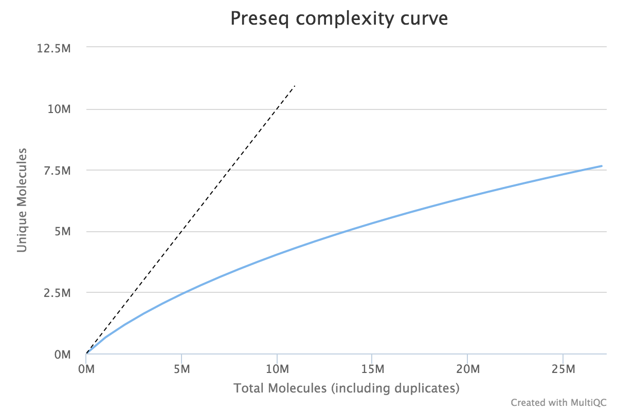
Lessons Learnt
Technical duplication is not always a simple thing to evaluate. It is not a good idea to blindly deduplicate samples since this can cause biases in itself, and a true estimation of technical duplication requires taking the local read density into account.
Software
The sequence level plots shown here were generated in FastQC and the plots of density vs duplication were done in SeqMonk. The density vs duplication plots can also be generated on the command line in DupRadar. The extrapolation of productive sequencing content can be done in Preseq with visualisation using MultiQC.
Mapping to a transcriptome can incorrectly report reads as mapping uniquely
Introduction
In the analysis of RNA-Seq data we often make an implicit assumption about our knowledge of the transcriptome in the species we’re working in. In some species the content of the transcriptome is very well understood and that information can be used to aid mapping. Some mapping programs such as Kallisto only map to a transcriptome and ignore reads which would map elsewhere in the genome. Other mappers such as TopHat employ a dual strategy where data is initially mapped to a transcriptome, and only goes on to map against the entire genome should no match be found within the transcriptome.
There is however a problem with these types of approach which revolves around the ability to define a read as uniquely mapping. For many analysis strategies it is easier and more accurate to deal only with reads which uniquely map to the reference so you can be sure that you are correctly assigning your signal. When mapping to a transcriptome though it is possible to have a read map uniquely within the transcriptome, but have it able to map to very many locations within the genome had such a mapping been performed. In many libraries these are purely theoretical concerns as the number of these reads is generally low, but where a significant amount of non-geneic transcription is present, or where DNA contamination occurs then these reads can drastically affect an otherwise robust analysis.
The Symptoms
This sort of artefact generally does not produce obvious symptoms initially. Overall metrics for the QC of the sample will not generally be adversely affected since the bias affects only a small number of genes. Even reviewing the data manually may not identify the problem. The problem is only really evident when reviewing some of the signficantly differentially expressed genes and looking at the distribution of the reads over the transcript. Normally you would expect that the reads would be relatively evenly distributed over the whole area of the transcript as shown below:
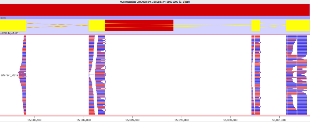
In a gene affected by this artefact the coverage would look very different, with a large number of reads mapping to a very limited region of the gene body. This would be the region which contained the repetitive sequence which is the underlying cause of this issue.
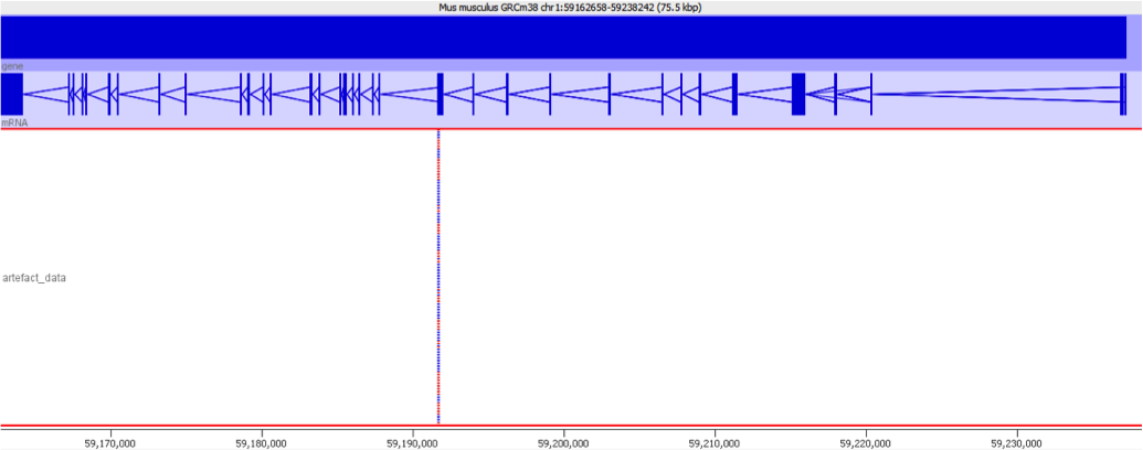
Diagnosis
When we encountered this issue we worked out the underlying cause by putting some of the aberrantly mapping reads through mapping with different mappers. We found that using a mapper which did not do an initial mapping to the transcriptome completely removed the signal which caused these genes to be selected initially.
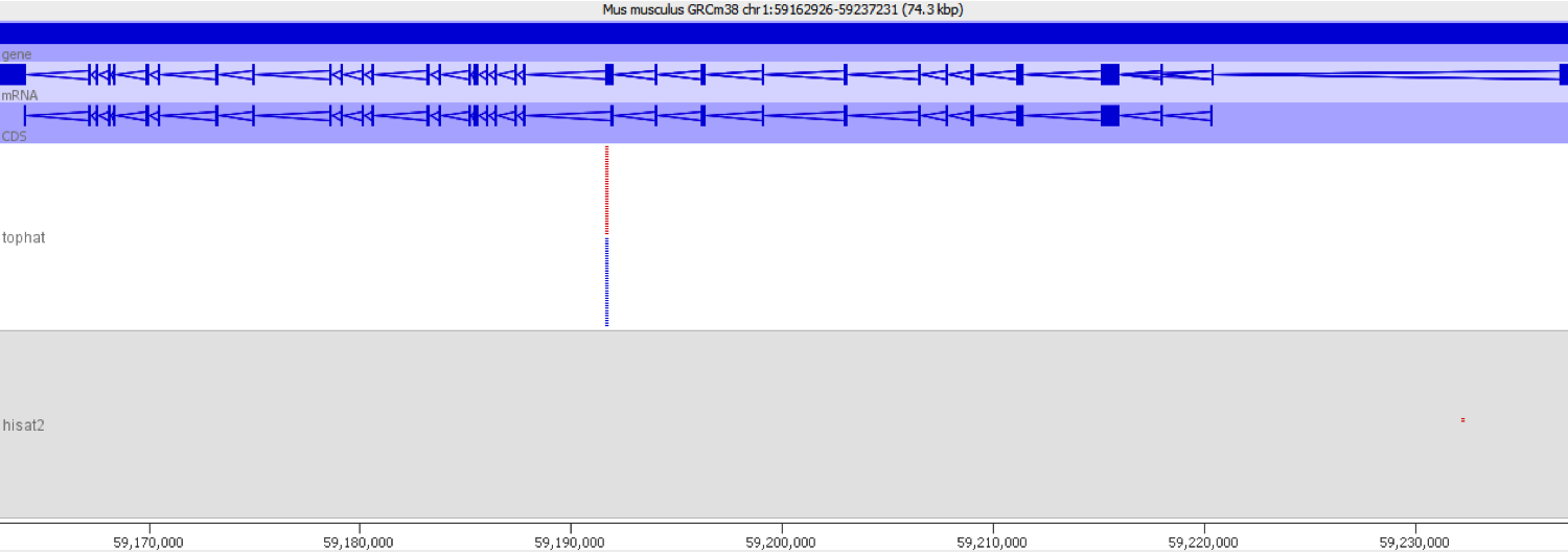
We also compared the quantitation produced by the two mappers used and found that there was a consistent bias for the transcriptome-first mapper to overestimate the expression relative to the whole genome mapper.
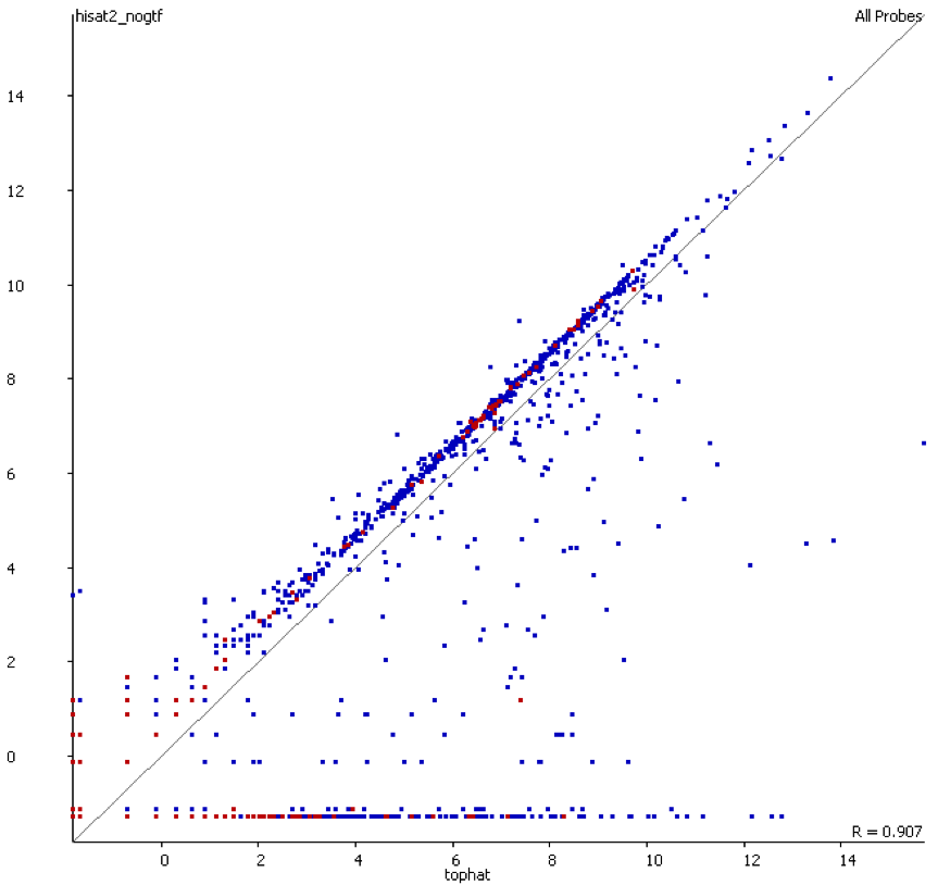
Mitigation
This issue was mitigated by re-mapping the data with the genome-first mapper and using this new mapper for the remainder of our RNA-Seq data.
Lessons Learnt
It’s always worth reviewing the hits you get from an analysis pipeline back through as far as the raw data to ensure that the signal you see comes in a form you would expect.
Software
The plots show here were all generated in SeqMonk.
The mapper which generated the artefacts was TopHat, the issue was reported to the TopHat developers, but the nature of the problem is such that there isn’t really a way to fix it without severely impacting the performance of the program.
The mapper which removed the artefacts was Hisat2, but we would expect that any other whole genome RNA-Seq mapper would have produced similar results.
RNA-Seq samples can be contaminated with DNA
Introduction
We generally think of contamination in samples coming from a completely external source such as a different sample or another species, but internal contamination is a real problem and can cause problems in the analysis of sequencing experiments. One of the most commonly seen internal contaminants is the presence of DNA in RNA-Seq samples. This type of contamination is very easy to miss and won’t generally trigger any errors in a standard RNA-Seq analysis pipeline, but can cause significant bias in the quantitated data.
Most RNA-Seq library preparation protocols include a DNAse treatment in the early stages to try to prevent the inclusion of any genomic material in the library. In practice it is not uncommon for the step to be ineffective and for DNA to make it through into the final library.
The Symptoms
Unless you specifically look for this type of contamination you will not generally see any specific symptoms from it. Mapping efficiency will generally not be too badly affected, and these reads will not trigger errors or warnings in any of the standard analysis pipelines. The inclusion of this data will however negatively impact the ability to correctly quantitate and normalise the data.
Diagnosis
DNA contamination is fairly easy to spot as long as you look for it. As soon as you visualise your reads against an annotated genome the presence of DNA is normally fairly apparent as a consistent background of reads over the whole genome which isn’t noticeable affected by gene boundaries. The reads should also have no directionality bias which makes them even easier to spot in directional libraries.
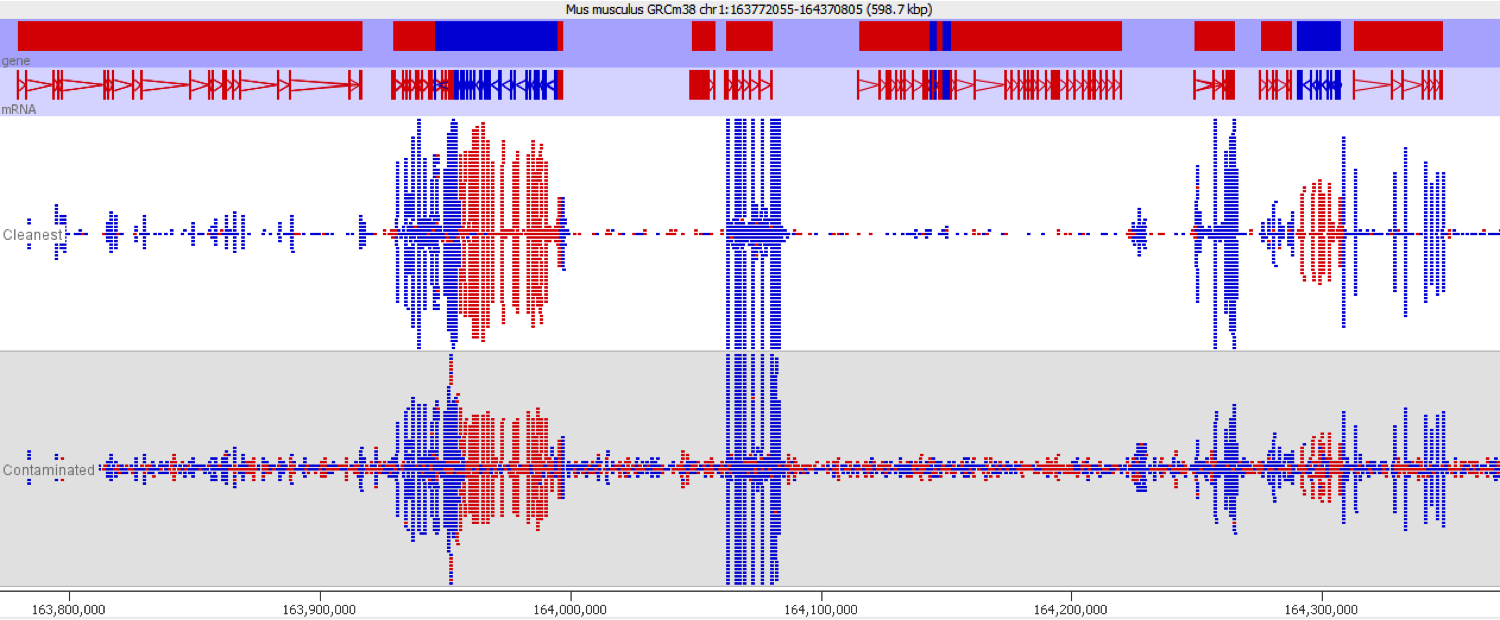
Since it isn’t always possible to visualise all datasets in large experiments you can also identify contamination by measuring some standard paramters such as the proportion of reads falling into genes, and the directionality of the reads.
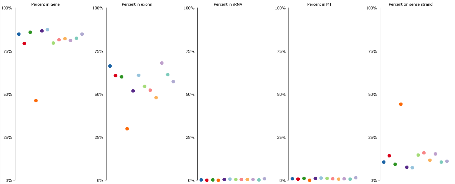
DNA contamination will also affect the quantitation of your data. If you compare the distributions of contaminated and non-contaminated samples then the contaminated samples will appear to have a loss of effective control on non-expressed genes which will all appear to be slightly expressed due to the random nature of the DNA derived reads. On more highly expressed genes the addition of DNA reads will have an insignificant effect, but the total number of reads involved can throw off global normalisation, and since the effect persists across a wide number of genes it can even throw off more robust normalisation schemes like size factor normalisation.
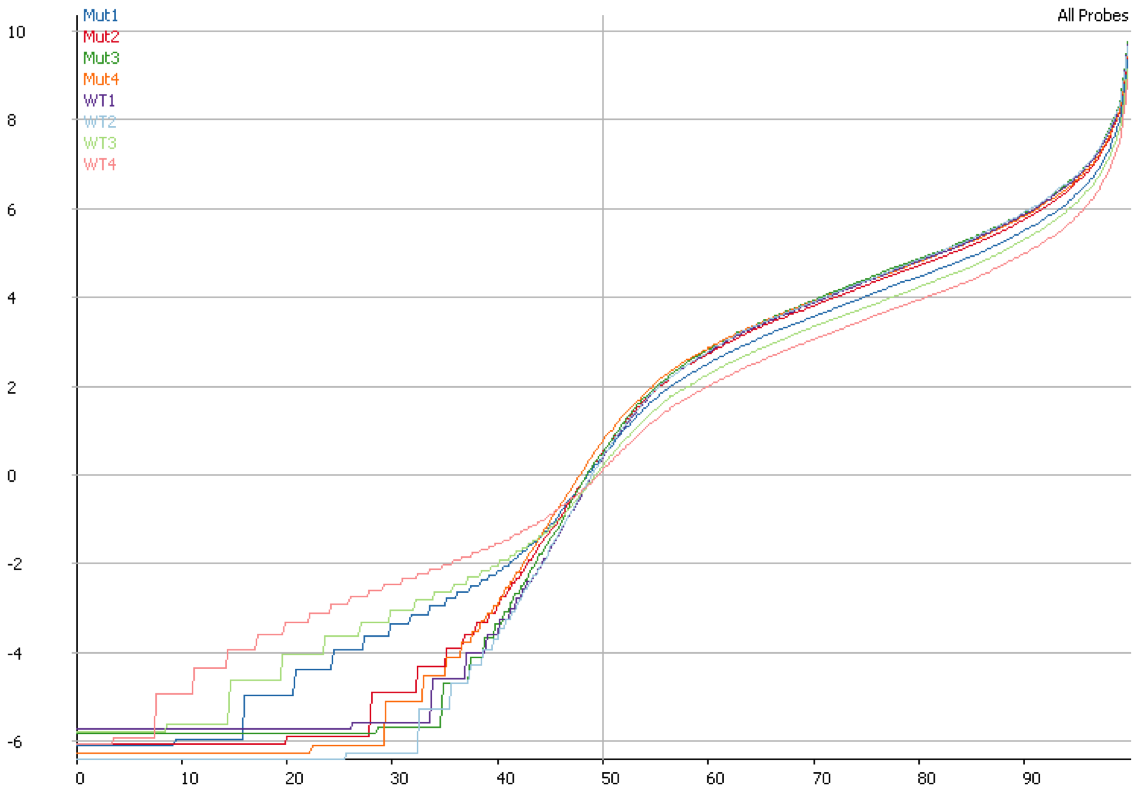
Mitigation
Once you have identified DNA contamination as an issue in your data it is possible to correct for it. In SeqMonk we use an option when we measure the median read density in intergenic regions over the genome on the assumption that this represents DNA contamination. This then allows us to estimate a per-transcript expected contamination level which can be subtracted from the observed count to try to get the DNA-free count. The plot below shows the quantitation for the same data shown in the previous plot after correcting for DNA contamination. It is clear that the overall distributions are much more closely matched after applying this correction.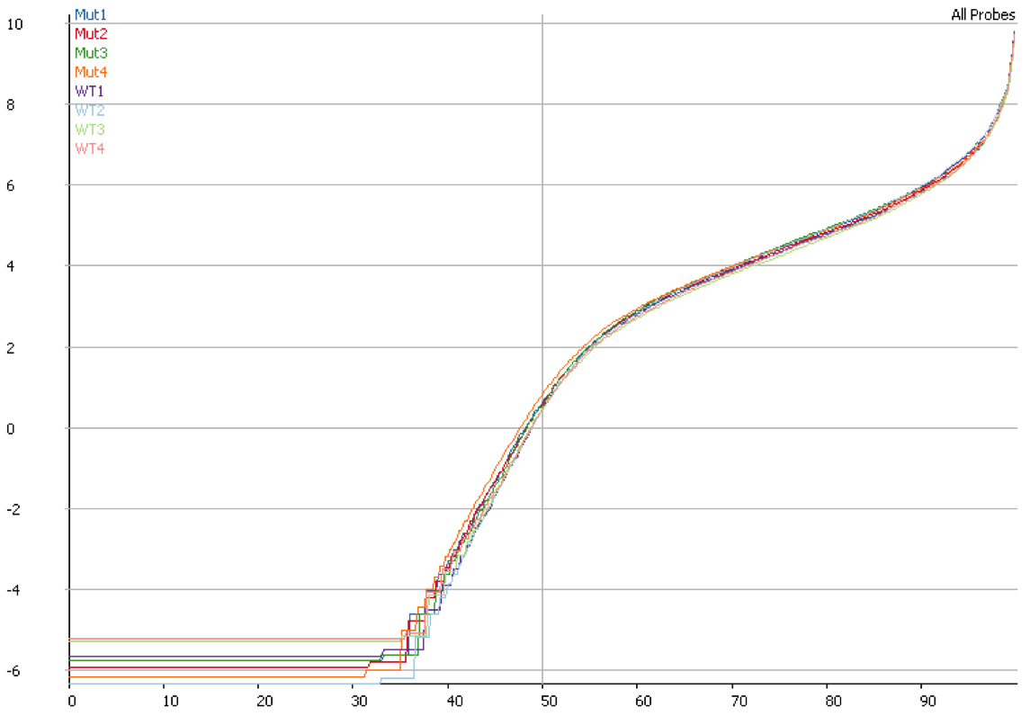
Prevention
This contamination can only be prevented at the library preparation stage through the rigorous use of DNAse treatment. Even then we regularly see instances of libraries with such contamination when such treatment was applied.
Lessons Learnt
Just because your pipeline runs smoothly doesn’t mean that there aren’t biases and artefacts in the data. Always find ways to view the key metrics for your raw and quantitated data.
Software
The plots in this article were all created with SeqMonk.
Contamination with a different species you can guess
Introduction
One common mode of failure for sequencing experiments is when mapping the sequence to the expected reference produces poor alignment efficiency. There are many potential reasons for this, but one of the most common is that some significant proportion (or possibly all) of the library comes from a species other than the expected one. Many times where material is from the wrong species, or is contaminated with a secondary species the contaminating species is one which is commonly used in the lab which created the library. It can therefore be useful to screen libraries across a range of commonly used species to determine the degree to which the library matches what is expected.
The Symptoms
Often the initial symptom observed would be a loss of mapping efficiency, but sometimes even the wrong species can map with reasonable efficiency and problems are not revealed until later in the analysis, so some pre-emptive QC on the libraries is useful.
In a simple case you should see the vast majority of the sequences mapping to the expected species.

This plot also illustrates that it can be useful to distinguish uniquely from multi-mapped reads. In this case the library is supposed to be mouse, but around 20% maps to Rat due to the overall similarity between the species. Separating uniquely and multiply mapped sequences allows us to quickly see that the rat mapped sequence is all multi-mapped and probably also maps to mouse. In an extreme case you could see what looks like reasonable mapping to the wrong species if the library is composed of sequences which are very easy to map (low complexity or short sequences for example).

Where there is significant contamination or a sample switch this type of screening will not only identity the problem, but will also provide a clue as to the source of the contamination and will say whether the library is completely the wrong species, suggesting a sample switch, or partially contaminated. The example below was supposed to be a mouse library, but can clearly be seen to be mostly E.coli but with some human sequence as well.

Lessons Learnt
It’s always worth investigating the whole content of your library. Even with partial contamination you will get some cross mapping to the species you expect from the contaminant and this can be difficult to spot if this type of screening is not run.
Software
The plots shown in this article were created with FastQ screen which is a program which can screen a proportion of your library against a set of species you select and can customise to match the environment you’re working in.
Contamination with adapter dimers
Introduction
The nature of many sequencing platforms is that their chemistry requires that specific adapter sequences are added to the end of the fragments to be sequenced. These adapters fulfil roles such as allowing for specific amplification and priming to support the underlying sequencing chemistry. Ideally a sequencing library should only contain valid adapter+insert constructs and manufacturers use a variety of techniques and modifications to try to ensure that these are highly enriched in the library.
However, it can happen that these precautions sometimes fail and a set of adapter dimers – a pair of ligated adapters with no insert sequence – end up in the library. These can still be sequenced because they contain all of the relevant parts of the sequencing template, but will produce no useful sequence. If these constructs end up present at high proportions of the library they can soak up significant amounts of the sequencing capacity in a lane and cause a number of QC metrics to be triggered.
The Symptoms
There are a couple of different ways to spot that this type of contamination has occurred. Because adapter dimers will always produce exactly the same sequence they will superimpose their sequence on the per-cycle base content plot. The example below is obviously extreme, but a reduced version of this pattern would appear in more modesty contaminated libraries.

The introduction of a number of identical sequences will also show up as a sharp spike in the overall GC profile for the run.

If you are monitoring over-represented sequences then this screen will also turn up this type of contamination since the sequences generated will be exactly the same each time, and will be present many thousands of times in the library.
Diagnosis
The easiest way to spot this is in the overrepresented sequences screen where the exact sequence will be shown and should be shown to match against the adapter sequence used. If the contamination is too low to trigger this module then you can normally see it as a fixed sequence super-imposed on the per base sequence content plot.
Mitigation
Adapter trimmers will generally remove this sort of data, but even without these the dimers do not normally map to a reference genome so don’t cause any further downstream disruption.
Prevention
Preventing this type of contamination must happen at the library preparation stage. Being careful about the amount of adapters added to the ligation mix, and being stringent on the size selection step for your library are going to be the most important parts for avoiding the formation and selection of dimers.